Quantcast
Channel: Analysis Services - Chris Webb's BI Blog
Viewing all 104 articles
Browse latest View live

How To Optimise The Performance Of MDX Queries That Return Thousands Of Rows

$
0
0

One problem I encounter on a regular basis is how to optimise the performance of MDX queries that return thousands, hundreds of thousands, or even millions of rows. The advice I give is always the same:

Reduce the number of rows that your query returns!

Yes, there are some things you can change in your queries and cube design to improve performance, but these are the same things I’d suggest for any query (build aggregations, rewrite MDX, partition etc etc). In my opinion, if you have a query that returns a ridiculously large number of rows you are doing something fundamentally wrong.

There are three reasons why SSAS developers write this kind of query:

  1. They are doing a data-dump from SSAS to another system. Mostly the developer doesn’t realise this though, since the other system is Excel-based and the end user has disguised their requirement as a report. In most cases, user education about how to use Excel with SSAS results in an approach that doesn’t require dumping thousands of rows of data to an Excel worksheet.I will admit that I have seen a few cases where developers need to dump data out of SSAS for other purposes, and have no option but to use SSAS because they have to add complex calculations that can only feasibly be implemented in MDX. These are very rare though, and most of the time using SQL queries against the underlying relational database works a lot better.
  2. The end users have specified a report that returns lots of data, because that’s just what they want, dammit! Often this is to recreate a report built in a previous system that, at some point in the 1970s, was printed out into a gigantic book every month. My argument here is that a report should return no more data than can be seen on a screen without scrolling. If you need to scroll in a report, you probably should be giving the end user more parameters to filter that report so they can find the data they want to see more easily instead.Of course it’s one thing to know what you should be doing, it’s another thing entirely to tell the CFO that their requirements are stupid. If you can’t convince your end users that you know better than them, you have my sympathy. Usually I find that having to choose between the poor performance of what they want and the better performance of a different approach helps them come to their senses.
  3. Finally, the way that SSRS handles drilling down in reports often leads report developers to bring back vast amounts of data. The advice to increase the number of parameters for filtering is equally relevant here, but you can also use MDX techniques like this one to implement drill down in a much more efficient way.

At the end of the day, SSAS just isn’t optimised for returning large resultsets – it was designed to return PivotTable-style queries, which are always relatively small. You can get good performance for large resultsets if you know what you’re doing, you have the time, and you’re lucky, but you’ll usually be better off rethinking your requirements or choosing a different tool.


What the MDX Axis() Function Actually Returns

$
0
0

A month or so ago, before I went on holiday, I was working on a really cool MDX idea that involved the Axis() function. Unfortunately I’ve forgotten what that idea was but while I was working on it I did find out something interesting about the Axis() function – namely that it doesn’t do exactly what the documentation says it does.
The documentation says that the Axis() function returns the set of tuples on a given axis in an MDX query. Here’s a simple example query on the Adventure Works cube showing it in action:

WITH
MEMBER MEASURES.TEST AS SETTOSTR(AXIS(1))
SELECT {MEASURES.TEST} ON 0,
[Customer].[Gender].MEMBERS ON 1
FROM
[Adventure Works]

image

Here, I’m using the SetToStr() function to take the set returned by the Axis() function and display it in a calculated measure. As you can see from the screenshot, I’m showing all three members from the Gender hierarchy on the Customer dimension on rows and the set returned by Axis(1) is indeed that set.

BUT, now look at this second query and what it returns:

WITH
MEMBER MEASURES.FIRSTMEMBER AS 
MEMBERTOSTR(AXIS(1).ITEM(0).ITEM(0))

MEMBER MEASURES.TEST AS 
IIF(
[Customer].[Gender].CURRENTMEMBER.UNIQUENAME = 
MEASURES.FIRSTMEMBER, NULL, 1)

SELECT MEASURES.TEST ON 0,
NON EMPTY
[Customer].[Gender].MEMBERS ON 1
FROM
[Adventure Works]

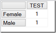
image

Why is this interesting? The calculated measure FIRSTMEMBER returns the unique name of the first member in the set returned by Axis(1), which should be the first member shown on the rows axis. The calculated measure TEST returns null if the currentmember on the Gender hierarchy has the same unique name as the member returned by FIRSTMEMBER. The calculated measure TEST is on columns in the query, and on rows we get all the members on the Gender hierarchy that return a non null value for TEST. Since only Female and Male are returned, the All Member on Gender must return null for TEST, which means that the All Member is the first member in the set returned by the Axis() function.

So, to summarise, the Axis() function actually returns the set of members on an axis the current query before any NON EMPTY filtering is applied.


Power BI And SQL Server 2016 BI Announcements At PASS Summit 2015

$
0
0

image1

This year’s PASS Summit is drawing to a close as I write this, and I have to say that the number of Microsoft BI-related announcements made over the last few days has been overwhelming. There have been announcements made via blog posts, such as (shock!) the roadmap blog post:
http://blogs.technet.com/b/dataplatforminsider/archive/2015/10/29/microsoft-business-intelligence-our-reporting-roadmap.aspx

…which you should probably read before anything else, as well as the following posts which have more details on specific areas:
http://blogs.technet.com/b/dataplatforminsider/archive/2015/10/28/sql-server-2016-community-technology-preview-3-0-is-available.aspx

http://blogs.msdn.com/b/analysisservices/archive/2015/10/28/what-s-new-for-sql-server-2016-analysis-services-in-ctp3.aspx

http://blogs.msdn.com/b/sqlrsteamblog/archive/2015/10/28/pin-reporting-services-charts-to-power-bi-dashboards-with-sql-server-2016-ctp-3-0.aspx

There have also been a lot of other announcements made in sessions about functionality that will be available at some point in the next few months, including (and in no particular order):

  • The performance problem with Excel subtotals that I described in this blog post: http://blog.crossjoin.co.uk/2011/10/07/excel-subtotals-when-querying-multidimensional-and-tabular-models/ is finally going to be addressed in Excel 2016 in an update that will be available before the end of the year. This is going to solve a lot of people’s performance problems – problems that people may not even realise they had.
  • SSDT for SSAS 2016 will have a script view where you can see all of your DAX calculations in one place
  • SSDT will be getting monthly updates so new functionality can be delivered much more quickly
  • On top of the improvements in SSAS Tabular DirectQuery mentioned in the blog posts above, we’ll also get support for row-level security and calculated columns (but only ones that reference values in the same row of the table that the calculated column is on)
  • SSAS Tabular will also get Translations, but only for metadata and not for data
  • There will be a Power BI Enterprise Gateway, the corporate big brother of the Personal Gateway
  • Datazen will be rolled into SSRS and Datazen reports will be a new ‘mobile’ report type
  • The Power BI mobile app will be able to display these new SSRS mobile reports as well as Power BI reports
  • The Power BI team will be releasing a new custom datavisualisation component every week. We had the new Chiclet slicer this week, which I am already using lots, and in one demo I spotted a Proclarity-style decomposition tree
  • Power BI desktop will work with SSAS Multidimensional as a live data source (ie not through importing data, but running DAX queries in the background) by the end of this year
  • PowerBI.com dashboard tiles will become properly interactive, and you will be able to pin entire reports as well as just individual components to them
  • You’ll be able to embed ranges and charts from Excel workbooks into PowerBI.com reports; integration looks much nicer than the rather basic functionality that’s already there
  • Power Map/3D maps will be embedded in Power BI Desktop and PowerBI.com
  • You’ll be able to run R scripts in Power BI Desktop and display R visualisations in there too
  • There was a demo of an Android(?) phone version of the Power BI mobile app, where when the phone camera saw a QR code it displayed a report for the product that the QR code represented over the camera feed. Virtual reality BI!
  • Power BI Desktop will get a “Get Insights” button that, when pushed, will display a report that does some basic statistical analysis of your data, looking for minimums, maximums, outliers etc
  • The Power BI API will be able to give you a list of reports and their URLs
  • Power BI will soon have its own registration page for applications that use the API; no need to go to the Azure Portal.
  • Synonyms and phrasings for Q&A will be coming to Power BI by the end of the year

I *think* that’s everything, but I may well have missed a few things. Many of the features that were mentioned in passing would have deserved a five-minute slot in a keynote in previous years.

Power BI is finally a commercially viable product and it’s getting even better every week – the competition should be very worried. I’m also really pleased that MS are taking corporate, on-premises BI seriously at last and that SSRS is back in favour (I would have loved more new features in SSAS Multidimensional, but hey, you can’t have everything) – if you’re wondering what the picture at the top of this post is, it’s the cloud and boxed SQL Server “happy together” at last, and it appeared in several MS presentations this week. The box is back! Most importantly, for the first time in a long time, Microsoft has a coherent vision for how all of its BI products should work together, it’s working on new features to make that vision a reality, and it is willing to share it with us as a roadmap.

In summary I can’t remember the last time I felt this positive about the future of Microsoft BI. What MS have achieved over the last year has been remarkable, and it seems like it’s the leadership of James Phillips that has made all the difference – every MS employee I’ve talked to has had good things to say about him and I guess this explains why he got a promotion in the reorg last week. I hope all this continues.


First Look At SSAS 2016 MDX On DirectQuery

$
0
0

Following on from my last post covering DirectQuery in Power BI, I thought it might be interesting to take a look at the way MDX queries are supported in SSAS Tabular 2016 CTP3 DirectQuery mode.

There were a lot of limitations when using DirectQuery in SSAS Tabular 2012/4, but for me the showstopper was the fact that it only worked if you were running DAX queries against your model. Historically the only major client tool that generated DAX queries to get data was Power View, and Power View was/is too limited for serious use, so that alone meant that none of my customers were interested in using DirectQuery. Although we now have Power BI Desktop and PowerBI.com, which also generate DAX queries, the fact remains that the vast majority of business users will still prefer to use Excel PivotTables as their primary client tool – and Excel PivotTables generate MDX queries. So, support for MDX queries in DirectQuery mode in SSAS 2016 means that Excel users will now be able to query a Tabular model in DirectQuery mode. This, plus the performance improvements made to the SQL generated in DirectQuery mode, means that it’s now a feature worth considering in scenarios where you have too much data for SSAS Tabular’s native in-memory engine to handle or where you need to see real-time results.

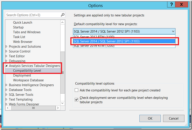
At the time of writing the most recent release of SQL Server 2016 is CTP3. If you want to test out the BI features in SQL Server 2016 CTP3 in an Azure VM, I highly recommend Dan English’s blog post here showing how to set one up. To test DirectQuery mode you need to use the older 1103 compatibility mode for your project and not the latest 1200 compatibility mode. This is documented in the release notes:
https://msdn.microsoft.com/en-us/library/dn876712.aspx#bkmk_2016_ctp3_0

image

Once you’ve created your project, you can enable DirectQuery mode in the same way as in previous versions by following the instructions here. The DirectQueryMode property on Model.bim needs to be set to On, and the QueryMode property on the project should be set to DirectQuery.

For testing purposes I downloaded the 2016 version of the Adventure Works DW database and restored it to SQL Server, then created a SSAS Tabular model containing only the DimDate table to keep things simple. I created one measure in the model with the following definition:
TestMeasure:=COUNTROWS(‘DimDate’)

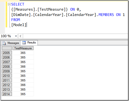
First of all, I ran the following MDX query:

SELECT
{[Measures].[TestMeasure]} 
ON 0,
[DimDate].[CalendarYear].[CalendarYear].MEMBERS 
ON 1
FROM
[Model]

image

Using a Profiler trace (yes, I know I should be using XEvents but Profiler is so much more convenient for SSAS) I could see the SQL generated by SSAS in the Direct Query Begin and Direct Query End events. For the MDX query above there were three SQL queries generated. The first looks like it is getting the list of years displayed on the Rows axis:

SELECT 
TOP (1000001) [t0].[CalendarYear] AS [c15]
FROM 
(
  (SELECT [dbo].[DimDate].* FROM [dbo].[DimDate])
)
AS [t0]
GROUP BY [t0].[CalendarYear] 

The second SQL query gets the measure value requested:

SELECT 
TOP (1000001) [t0].[CalendarYear] AS [c15],
COUNT_BIG(*)
AS [a0]
FROM 
(
  (SELECT [dbo].[DimDate].* FROM [dbo].[DimDate])
)
AS [t0]
GROUP BY [t0].[CalendarYear] 

The third is simply a repeat of the first query.

However, there’s one important thing to say here: there are going to be significant changes and improvements to the SQL generated before RTM, so don’t read too much into the queries shown here.

There are several limitations in CTP3 that may or may not remain at RTM. One that you may run into is the that you can only use fully qualified MDX unique names in your queries, so

[DimDate].[CalendarYear].&[2010]

…will work but

[2010]

…will not. To be honest, I consider it a best practice to use fully qualified unique names anyway so I’m not too bothered about this. Drillthrough doesn’t work at the moment either.

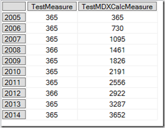
MDX calculations defined in the WITH clause of a query are supported, which is really useful if you’re writing custom MDX queries for SSRS. For example the following query works and generates the same SQL (though with a few more executions) as the previous query:

WITH
MEMBER [Measures].[TestMDXCalcMeasure] AS 
SUM(NULL:[DimDate].[CalendarYear].CURRENTMEMBER,
[Measures].[TestMeasure])

SELECT
{[Measures].[TestMeasure],
[Measures].[TestMDXCalcMeasure]} 
ON 0,
[DimDate].[CalendarYear].[CalendarYear].MEMBERS 
ON 1
FROM
[Model]

image

All in all, this looks like a solid piece of work by the SSAS dev team. Go and test it! I would love to hear from anyone with genuinely large amounts of data (maybe APS/PDW users?) regarding their experiences with 2016 DirectQuery. Recently I’ve been working with a customer using SSAS Multidimensional in ROLAP mode on top of Exasol and I’ve been surprised at how well it works; I would imagine that 2016 DirectQuery and APS would be an even better combination.

One last thought. If we get the ability to query a cloud-based Power BI mode with MDX and MDX on DirectQuery is supported in Power BI too, why would you bother paying for an expensive SQL Server Enterprise/BI Edition licence plus hardware to use DirectQuery when you can get almost the same functionality in the cloud for a fraction of the price?


Webinar Recording: Is OLAP Dead?

$
0
0

Yesterday I presented a webinar for the nice people at Pyramid Analytics, the first of two. I was paid for it of course (I have to earn a living somehow, you know), but the main reason I agreed to do it was because they wanted me to discuss interesting Microsoft BI questions rather than just demo their product – which is, as I’ve said here before, the most effective way of doing tech marketing in my opinion. In any case Pyramid Analytics is one of a small number of third-party tools I’m happy to recommend to my customers even without being paid.

Today’s discussion was on the topic of whether OLAP is dead and you can watch the recording here: https://www.brighttalk.com/webcast/13401/178899 [free sign-up required]

You won’t be surprised to find out that I don’t think OLAP is dead. By “OLAP” I mean the idea of a centralised model containing not just all your data but also things like how your tables should be joined, how measures aggregate up, advanced calculations and KPIs and so on. Using this definition both SSAS Multidimensional and SSAS Tabular are OLAP; I would say both pass the FASMI test for sure. The opposite of OLAP is of course the recently-fashionable self-service BI approach of tools like Power Pivot where every end user can create their own model, which is certainly more flexible but also less easily maintainable, leads to duplication of effort and data, and can be a problem for less technically-able end users. Both a single centralised OLAP model and a distributed self-service approach are useful in different circumstances and the latter certainly doesn’t replace the former. One of the reasons why I’m such a fan of Microsoft’s new direction with Power BI is that it recognises this fact.

The other big question that came up was what the relative strengths and weaknesses of SSAS Multidimensional and Tabular are. Before the webinar I ran a Twitter poll asking people whether they had used Multidimensional or Tabular on the last SSAS project that had worked on; from 151 responses, 48% said Tabular and 52% said Multidimensional. This even split doesn’t surprise me to be honest, based on my own experiences: both flavours of SSAS have different strengths and weaknesses and choosing between them can be very difficult. I’m sure new features like bi-directional cross-filtering and the improved development experience in SSAS Tabular 2016 will increase Tabular’s popularity in the future. Personally, I think if Microsoft were able to offer equivalent functionality to:

  • Calculated members on non-measures dimensions
  • MDX SCOPE statements
  • Parent/child hierarchies (without the performance penalties)
  • Writeback

…in SSAS Tabular then there would be very few good reasons to choose SSAS Multidimensional for new projects.


New SSAS, Power BI And SQL Server Training Courses For 2016

$
0
0

I’ve just added a number of new 2016 training course dates to the Technitrain site. If you’re looking for Power BI, Analysis Services, SQL Server or Data Science training in London then please check them out! Also, if you’d like to sign up for the Technitrain newsletter to stay up-to-date with our news you can do so here.

Here are more details on the new courses:

SQL Server Performance Tuning and Internals Boot Camp, Bradley Ball, 15-19 February 2016, London
This 5-day hands-on course is designed to provide DBAs with the tools and knowledge that are required to keep their SQL Servers running efficiently and reliably.
http://technitrain.com/coursedetail.php?c=60&trackingcode=CWB

Introduction To Power BI, Chris Webb, 22-23 February 2016, London
A two-day introduction to Microsoft’s exciting new BI tool suitable for BI professionals, analysts, report developers or anyone interested in using it to build reports or dashboards.
http://technitrain.com/coursedetail.php?c=65&trackingcode=CWB
 
Real World Cube Design And Performance Tuning With SSAS Multidimensional,  Chris Webb, 11-13 April 2016, London
A course aimed at intermediate-to-experienced Analysis Services Multidimensional developers, looking at more advanced cube design topics and query performance tuning.
http://technitrain.com/coursedetail.php?c=66&trackingcode=CWB

Mastering DAX, Marco Russo, 20-22 June 2016, London
A three-day introduction to the DAX language used by Power BI, Analysis Services Tabular models and Power Pivot.
http://technitrain.com/coursedetail.php?c=63&trackingcode=CWB

Optimising DAX, Marco Russo, 23-24 June 2016, London
An advanced two-day course for experienced DAX developers who wish to learn how to optimise DAX calculations and queries for performance.
http://technitrain.com/coursedetail.php?c=64&trackingcode=CWB

Introduction to MDX, Chris Webb, 4-6 July 2016, London
A three day course designed for those with little or no experience of MDX, this course will teach you how to write MDX queries and calculations for Analysis Services.
http://technitrain.com/coursedetail.php?c=67&trackingcode=CWB
 
Practical Data Science with Cortana Analytics, Rafal Lukawiecki, 24-27 October 2016, London
This course is aimed at analysts, analytical power users, predictive developers, BI power users and developers, budding data scientists and consultants.
http://technitrain.com/coursedetail.php?c=68&trackingcode=CWB


Two New Books: “The Definitive Guide To DAX” And “’M’ Is For Data Monkey”

$
0
0

I’m not going to pretend that this blog post is a properly impartial review – I know the authors of both of these books to varying degrees – but I thought it was worth writing a few words on two new books I’ve acquired recently which are worth additions to any Power BI enthusiast’s bookshelf or e-reader.

The Definitive Guide To DAX

Something I’ll never understand about my friends Marco Russo and Alberto Russo is their love of writing books – they generally have a new one out every year, sometimes two (personally I find writing books painful). Their latest publication is “The Definitive Guide To DAX” and it does indeed live up to its title. No-one outside the dev team comes close to Marco and Alberto’s knowledge of DAX, the language of Power Pivot, Power BI Desktop modelling and SSAS Tabular, and in this book they have documented everything that they know about it down to the smallest detail. Want to know what the KeepFilters() function does? Or the GenerateAll() function? How about all the new DAX functions and features in the latest versions of Power BI Desktop which will also appear in SSAS 2016 Tabular? They’re all here, and more. As such this is essential purchase for anyone doing serious work on the Microsoft BI platform, although probably more as a reference than a book to read end-to-end. It’s fair to say there’s a certain amount of overlap between this and some of their previous books on Power Pivot and SSAS Tabular, but the language – and the community’s understanding of it – has evolved sufficiently to justify buying this book too.

[I received a free copy of this book for review]

Buy it here from Amazon UK | US

‘M’ Is For Data Monkey

As the author of the only other book on Power Query, I suppose I should really be keeping quiet about “’M’ Is For Data Monkey” in case you buy it instead of mine. However 18 months of UI changes and functionality improvements mean my book is now a bit out-of-date, and what’s more important is that Ken Puls and Miguel Escobar have had the advantage of a lot of real-world experience with Power Query that I didn’t have (indeed no-one had) when I was writing in early 2014. The book itself is not a formal introduction to the M language but a guide to what you can do with it in Power Query; while a lot of what’s here will be useful in Power BI this is definitely a Power Query book and the target audience is Excel Pros rather than BI Pros. The decision to focus on Excel Pros was a good one to make, in my opinion, because it plays to the authors’ strengths and means that the book has a very practical focus. A lot of the tips and tricks here are ones I’ve used successfully myself, and I don’t mind admitting that I learned one or two things from this book as well.

Buy it here from Amazon UK | US

Other Books Are Available…

There are a couple of other new books out that, although I haven’t seen them, will also be worth checking out. Rob Collie has just released Power Pivot and Power BI, essentially the second edition of DAX Formulas For Power Pivot; Matt Allington has just released Learn To Write DAX; both are going to be good choices for Excel users wanting a DAX tutorial. Finally, last week Teo Lachev announced on his blog that he has published the world’s first dedicated Power BI book. Teo is another author whose books I admire so I’m sure it will be excellent, although I’ll be interested to see how he handles the problem of writing about a product that changes so much so quickly.


Monitoring SSAS Multidimensional MDX Query Results Serialisation, Part 1

$
0
0

Profiler (or indeed XEvents) can tell you a lot of interesting things about what happens when SSAS Multidimensional serialises the resultset returned by an MDX query. To be honest, this isn’t something I’ve looked at in detail before but recently I decided to do some research in this area – it turns out that monitoring the Profiler events related to serialisation can be very useful when you’re trying to understand what a Profiler trace is telling you about query execution as a whole.

To start off, let’s look at some very simple examples. Consider the following MDX query on the Adventure Works DW database:

SELECT
{[Measures].[Internet Order Quantity],
[Measures].[Internet Sales Count]}
ON 0,
[Date].[Calendar Year].[Calendar Year].MEMBERS
ON 1
FROM
[Adventure Works]

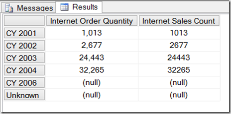
If you run it in SQL Server Management Studio in an MDX query window, you’ll get the following cellset back:

image

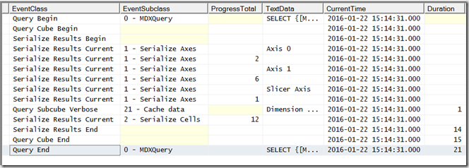
Running a Profiler trace using, amongst others, the Serialize Results Begin, Serialize Results Current and Serialize Results End events shows how SSAS is constructing the cellset returned:

image

The Serialize Results Begin event marks the point where SSAS starts to construct the cellset returned. The Serialize Results Current events that immediately follow it, with EventSubclass “1 – Serialize Axes” show SSAS serialising the tuples that are present on the Columns axis (listed as Axis 0 in the TextData column), the Rows axis (Axis 1) and the Where clause (Slicer Axis). The numeric values in the ProgressTotal column for the Serialize Results Current events shows the number of tuples on each axis: the two tuples on columns are the two measures, the six tuples on rows are the six years, and there’s one tuple on the slicer. After that SSAS gets the data for each of the cell values (as shown by the Query Subcube Verbose event – note that this query is running on a warm cache) and there is then a Serialize Results Current event with EventSubclass “2 – Serialize Cells”; the ProgressTotal column shows that twelve cells (2 columns * 6 rows) in total were returned.  The Serialize Results End event shows that SSAS has finished constructing the cellset and not surprisingly it’s followed immediately by the Query Cube End and Query End events.

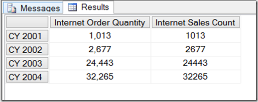
Sometimes SSAS needs to do a bit more work to find out what tuples are on an axis before serialisation can begin. The following query adds a NON EMPTY to the rows axis of the query above, so that only the rows that have values are returned:

SELECT
{[Measures].[Internet Order Quantity],
[Measures].[Internet Sales Count]}
ON 0,
NON EMPTY
[Date].[Calendar Year].[Calendar Year].MEMBERS
ON 1
FROM
[Adventure Works]

image

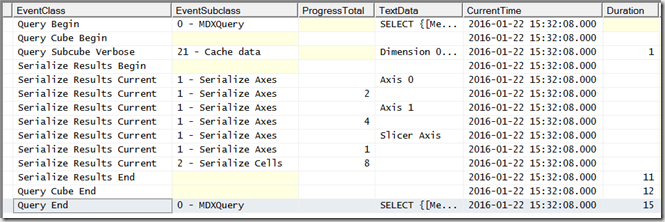
In order to know which years will appear on rows it has to query the cube to find out which ones have values for the measures on columns; as a result the Profiler trace shows a Query Subcube Verbose event appearing now before Serialize Results Begin:

image

This trace deliberately doesn’t show any of events related to the NON EMPTY operation (something I’ll be writing about in future blog posts), but it looks like SSAS can work out which years have values and get the values needed for the cellset back in a single operation so there’s no need for another Query Subcube Verbose event before the Serialize Cells event. Note that now the empty rows have been excluded, the ProgressTotal shows that only four tuples are returned on rows and eight cells are returned overall.

Cellsets are not the only type of resultset that SSAS can return though. Some client tools, most notably Reporting Services, return a tabular dataset that doesn’t have the concept of axes; running the previous query in SSRS gives the following in Profiler:

image

As you can there is now only one Serialize Results Current event and it has the EventSubclass “3 – Serialize SQL Rowset” (even though this is still an MDX query); the ProgressTotal column shows four, which is the number of rows returned.

In Part 2, I’ll look at what happens when a query returns a much larger amount of data.


Monitoring SSAS Multidimensional MDX Query Results Serialisation, Part 2

$
0
0

In part 1 of this series I looked at the basics of monitoring SSAS Multidimensional query resultset serialisation in Profiler. In this post, I’ll be taking a look at what happens for queries that return large amounts of data

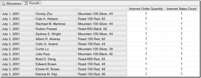
Consider the following query on the Adventure Works DW database, which, when I run it in SQL Server Management Studio returns a cellset with 60391 rows:

SELECT
{[Measures].[Internet Order Quantity], 
[Measures].[Internet Sales Count]}
ON 0,
NON EMPTY
[Date].[Date].[Date].MEMBERS
*
[Customer].[Customer].[Customer].MEMBERS
*
[Product].[Product].[Product].MEMBERS
ON 1
FROM
[Adventure Works]

image

There are a couple of interesting things to note about this query. First, SQL Server Management Studio on my laptop says that it takes nine seconds to run, even on a warm cache; the Duration column for the Query End event in Profiler, however, shows a value of around six seconds. The three second difference must be the time it takes for SSAS to return the cellset to SQL Server Management Studio, and for SQL Server Management Studio to render the results (my guess is that it’s the second operation that takes the majority of this time – other client tools may be more efficient at rendering large resultsets).

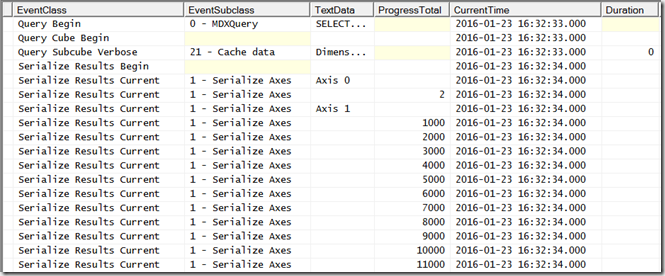
Secondly, in Profiler, you’ll see a much larger number of Serialize Results Current events. In situations where an axis contains more than a thousand tuples, or a cellset contains more than a thousand cells, you’ll see one Serialize Results Current event for each thousand tuples or cells. The ProgressTotal column will show values incrementing by one thousand up to the total number of tuples or cells. So, here’s some of what Profiler shows for the serialisation of the Rows axis:

image

…and here’s the end of the trace, showing the end of the serialisation of the cells (60391 rows * 2 columns = 120782 cells):

image

The third thing to notice is that there is only one Storage Engine operation – shown by the Query Subcube Verbose event in the first Profiler screenshot above – and that hits the Storage Engine cache and is so quick the Duration column shows 0 ms. Getting the raw data isn’t the problem here, and there aren’t any MDX calculations either – which means that it’s the Non Empty filter and construction of the cellset that is taking all the time. Since neither of these operations can be cached (although you can play tricks like this), this explains why the query always takes six seconds to run, even on a warm cache. Further investigation reveals that the Non Empty filter in fact only takes about a quarter of a second, so it’s the construction of a large cellset that’s the real problem here. This is why I say you should always avoid queries that return large amounts of data! SSAS is not very good at returning large resultsets.

Incidentally, don’t fall into the trap of thinking that the values shown in the Duration column for the Serialize Results End event only represents the amount of time taken to construct the cellset. It shows the amount of time since the Serialize Results Begin event, and in between the Begin and End events all kinds of other things necessary for the query to return (such as the evaluation of MDX calculations) could be going on. In a lot of cases the Serialize Results End event shows a duration that is almost the same as the duration for the whole query, but that only means that serialisation was able to start soon after the query began. In order to find the overhead of serialisation you need to work out how long all these other things take and subtract that from the duration shown for Serialize Results End, and that’s easier said than done.

Finally, what can you do to improve performance? Well, in the first post in this series I showed there was a tabular alternative to a cellset, and this is certainly a lot more efficient at returning large amounts of data (although you probably won’t have a choice in this unless you are building your own client tool, and, SSRS uses the tabular format anyway). For this query a tabular resultset is almost two seconds faster to return than a cellset, at just over four seconds:

image

There’s another important technique you can use, once that I have already mentioned in a blog post a couple of years ago but which is worth mentioning again: each cell returned by this query returns a large number of properties that you may not need, and these extra properties have a significant effect on the size of the resultset. Adding a CELL PROPERTIES clause to the query so that you only return the value property, like so:

SELECT
{[Measures].[Internet Order Quantity], 
[Measures].[Internet Sales Count]}
ON 0,
NON EMPTY
[Date].[Date].[Date].MEMBERS
*
[Customer].[Customer].[Customer].MEMBERS
*
[Product].[Product].[Product].MEMBERS
ON 1
FROM
[Adventure Works]
CELL PROPERTIES VALUE

…takes another two seconds off the duration of the query, whether you use a tabular resultset or a cellset:

image


Disabling Excel PivotTable Grouping And Session Cubes In SSAS Multidimensional

$
0
0

The Excel PivotTable grouping functionality that is available when you are connected to an SSAS Multidimensional cube (but not a Tabular model) is a Very Bad Thing indeed. In my experience it is a major cause of query performance problems – not just for the person running the query, but because it is so resource intensive for everyone else trying to query the cube too. This post from a few years ago gives some more details about why custom grouping, and the CREATE SESSION CUBE MDX statements that it uses behind the scenes, are so expensive.

Up until now it was impossible to prevent users from using custom grouping but in a recent cumulative update this changed. First of all, I encourage you to read the details of the fix because you will probably want to install the relevant CU for security reasons anyway:

https://support.microsoft.com/en-us/kb/3080856

[And if you are wondering whether you should be installing CUs I strongly suggest you read this post by Aaron Bertrand]

Once the CU has been installed the following new property is added to the msmdrv.ini file:

\OLAP\Query\SessionCubesMode

This will be set to 1. Setting this property to 0 will prevent users from creating session cubes and therefore prevent them from using Excel’s custom grouping functionality.

My opinion is that it’s a good idea to disable session cubes and custom grouping even if you don’t know whether your users are using these features. Yes, your users will lose some functionality and some reports might even break, but you will also save yourself and your users a lot of problems. If your users need to do custom grouping in a report that is usually an indication that you have missed something in your dimension design, and that an extra attribute hierarchy or two is necessary.

[Thanks to Akshai for this information]


Finding All Selected Items In A Slicer In Excel 2016 Using TextJoin()

$
0
0

When you are using slicers with an Excel PivotTable it’s often useful to be able to get a comma-delimited list of the items selected in that slicer for use in a report title. It’s not easy to do though, and in fact this is one of those topics that lots of people have blogged about over the years: here’s my MDX approach, here’s Erik Svensen’s post on using the new DAX ConcatenateX() function, and there are also posts by Rob Collie like this one. None of these techniques are ideal though: my personal favourite is the ConcatenateX() approach, but that only works with SSAS Tabular 2016 (and then only if you can create a measure on the model) or Power Pivot in Excel 2016, and not at all if you’re using SSAS Multidimensional or earlier versions of SSAS Tabular.

However, after discovering the new TextJoin() function in Excel 2016 the other week I realised that this would provide yet another way to solve this problem. Here’s a simple example using a PivotTable and slicer connected to a Power Pivot model:

image

The highlighted cell F3 showing a comma-delimited list of all the items selected in the slicer has the following Excel formula:

=TEXTJOIN(
    ", ",
    TRUE,
     IFERROR(
      CUBERANKEDMEMBER(
        "ThisWorkbookDataModel",
        Slicer_Product,
        ROW(
         INDIRECT("1:"&CUBESETCOUNT(Slicer_Product))
        )
       ), 
      "")
     )

Important: this needs to be entered as an array formula, so instead of hitting Enter after typing in the formula you need to hit Ctrl+Shift+Enter. You’ll see the formula surrounded by braces {} in the formula bar when you do this:

image

image

This formula relies on the fact that the selection in a slicer (in the example above the slicer has the name Slicer_Product) can be treated the same as the output of the Excel CubeSet() function, which means that you can use the CubeSetCount() function to find the number of items selected and the CubeRankedMember() function to get the name of any single item in the selection. It also uses the Row()/Indirect() trick described here to create an array of numbers from 1 to the number of items selected in the slicer, which in turn provides the rank values to pass to the CubeRankedMember() function.

The beauty of this approach is that it works for Power Pivot and all versions of SSAS Tabular and Multidimensional, and doesn’t require any measures to be created on your models/cubes. It even works in Excel Online, so it will work inside Power BI, although it doesn’t seem to be possible to create array formulas in Excel Online yet so you need to create the formula on the desktop before you deploy. Of course you need the latest build of Excel 2016 for all this to work, and at the time of writing most people don’t have Excel 2016 and even if they do they probably won’t have a build (Version 16.0.6568.2025 or higher) with TextJoin() in it yet. But this will be a great solution in the distant future when everyone has Excel 2016, I promise!

You can download the sample Excel 2016 workbook here.

I also have to acknowledge the help of David Hager in writing this formula – we had a conversation about how TextJoin() behaves in array formulas in the comments of my earlier post and in doing so he provided the basic approach for me.


A Quick Look At Azure Data Catalog

$
0
0

I’ve been meaning to look at Azure Data Catalog for a long time but somehow never got round to it until now. I’m not sure why – perhaps it’s because there’s so much other cool stuff happening in the world of Power BI and Azure, and Azure Data Catalog seems a bit, um, boring in comparison. Maybe it’s a bit too much like documentation and all that other stuff we instinctively try to avoid. Whatever the reason, now I have looked at it I’m impressed and I can see its uses, not just for Power BI but also for traditional corporate BI scenarios. It certainly deserves a lot more attention from the Microsoft BI community than it seems to be getting at the moment.

First of all, what is Azure Data Catalog anyway? There’s lots of good documentation, videos and a tutorial here:
https://azure.microsoft.com/en-us/documentation/services/data-catalog/

…but the short answer is that it’s a cloud based service for cataloguing all the data sources you want to use for BI. It doesn’t store any of the data itself (except for a small amount for preview purposes, and you can turn that off), just the connection details; it also stores metadata (column names, data types etc) as well as descriptions, documentation and contact details for people who own or know about the data. End users can search the catalogue for data and even, for some data source types like SSAS, click a button to open that data source directly in Excel or Power BI Desktop.

image

Is it any good? Well, I managed to get going with it very easily. As well as an Azure subscription it does require you to have Azure Active Directory set up though, which is a pain – some of my customers (mostly the ones that have bought into Office 365 and Power BI) have it already, but I know for others it would be a showstopper. After setting everything up I was able to register SQL Server, SSAS and other types of data source very quickly using both the desktop application and the browser interface. It’s certainly simple enough for a reasonably technical end user to use and the implementation is very solid. I do have a few minor quibbles (I found the search results interface slightly confusing at first but soon came to grips with it) and it’s clear that it’s still very much a work in progress (right now the browser interface supports registering more data types than the desktop app, for example) but nothing very significant.

There is an obvious need for Azure Data Catalog if you are going to use Power BI and have embraced the whole concept of self-service BI: it makes it much easier for your users to find and consume the various different data sources that you have available. However, as I said earlier, I think on-premises users of SSAS and SSRS could also benefit from it too. It’s becoming increasingly common for me to see organisations with several SSAS cubes in production across various servers, each of them with a confusing list of measures and dimensions. Equally I’ve seen plenty of SSRS implementations with hundreds of reports, with nobody knowing what many of these reports do or even if they are used at all. Azure Data Catalog could provide a convenient central place to document and discover these cubes and reports. I guess it all depends on whether you can be bothered to do this documentation and annotation though, rather than whether you have a suitable tool for this purpose; I don’t think many organisations can be bothered, unfortunately.

One last thing: Azure Data Catalog is meant to include replacement functionality for the old Power BI for Office 365 Data Catalog but as yet it doesn’t allow you to publish or share Power Query queries. This is something that I and other Power Query/Power BI fans would love to see, especially if (unlike the old Data Catalog) it let you publish updates to your code without needing to manually update each Excel workbook/Power BI report that used it afterwards.


Monitoring SSAS Multidimensional Non Empty Filtering Using Profiler, Part 1

$
0
0

Filtering out empty values is something that SSAS does a lot of during query execution, and it is also a common cause of performance problems. In this series of posts (similar to my series earlier this year on results serialisation) I’ll look at the different types of non empty filtering that can occur in an MDX query, how they can be monitored using Profiler and what you can do to improve their performance.

Some of this information has come from an old white paper, but I’ve found that some of what that paper says is now out of date and I’m extremely grateful to Akshai Mirchandani of Microsoft for answering my questions on this subject. Even with the long-suffering Akshai’s help a lot of the information here is based on my own research and therefore potentially incomplete/inaccurate, potentially different for different versions of SSAS (I’m using SSAS 2014 for this series) and could potentially change again in the future, so take due care!

The first question to ask is: what counts as non empty filtering? There are actually several different operations that the engine treats as a non empty filter, a few of which I was surprised by; here are the ones I know about.

1) The NON EMPTY statement

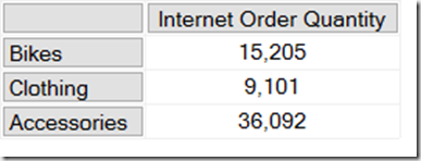
Most MDX queries generated by client tools include a NON EMPTY statement on the rows and columns axis. For example, take a look at the results returned by this MDX query on the Adventure Works cube:

SELECT 
{[Measures].[Internet Order Quantity]} 
ON 0,
[Product].[Category].[Category].MEMBERS 
ON 1
FROM
[Adventure Works]

image

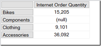
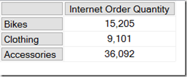
As you can see, the Product Category Components has no data and returns a null. One way to remove the row for Components would be to add a NON EMPTY statement to the rows axis:

SELECT 
{[Measures].[Internet Order Quantity]} 
ON 0,
NON EMPTY
[Product].[Category].[Category].MEMBERS 
ON 1
FROM
[Adventure Works]

image

2) The NONEMPTY() function

Often confused with the NON EMPTY statement, but not the same thing: the NON EMPTY statement can only be used on an axis in a SELECT statement, whereas the NONEMPTY() function can be used in any MDX expression. Continuing our example, here’s how to use it to remove the Component category:

SELECT 
{[Measures].[Internet Order Quantity]} 
ON 0,
NONEMPTY(
 [Product].[Category].[Category].MEMBERS,
{[Measures].[Internet Order Quantity]})
ON 1
FROM
[Adventure Works]

The NONEMPTY() function is much more flexible than the NON EMPTY statement but essentially does the same thing – it isn’t any faster in what it does, but it does allow you to make certain assumptions about your data that can improve query performance (more of that later). One thing to remember is to always set the second parameter, because if you don’t you may get unexpected results.

There is also a NONEMPTYCROSSJOIN() function but it is deprecated and you should not be using it – everything that it does can be done more reliably with other functions.

3) Autoexists

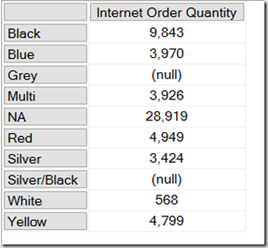
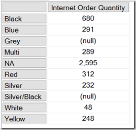
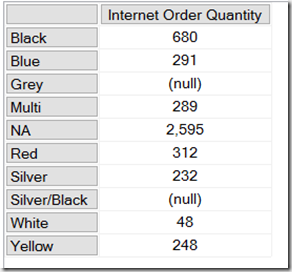
Autoexists is not a feature of the MDX language but rather something that SSAS does automatically to remove tuples from a set that it knows must always be null. It’s described in great detail here, but it’s quite easy to illustrate. We already know from the queries above which categories have data; similarly the following query shows there is data for all colours except Grey and Silver/Black:

SELECT 
{[Measures].[Internet Order Quantity]} 
ON 0,
[Product].[Color].[Color].MEMBERS
ON 1
FROM
[Adventure Works]

image

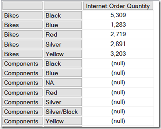
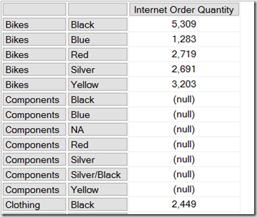
However if you crossjoin every category and every colour on the rows axis, you don’t see every combination of category and colour returned:

SELECT 
{[Measures].[Internet Order Quantity]} 
ON 0,
[Product].[Category].[Category].MEMBERS
*
[Product].[Color].[Color].MEMBERS
ON 1
FROM
[Adventure Works]

image

There is no row for the category Bikes and the colour White, for example. This is because the SSAS engine knows from the data in the dimension that no product exists that is both the colour White and in the category Bikes, so it doesn’t return that combination from the crossjoin – that particular tuple could never contain any data so there’s no point returning it. Notice that there are combinations, such as Components/Black, that exist in the dimension and are present on the rows axis but still return null because there is no value for Internet Order Quantity.

It’s important to remember that autoexists only takes place when you are working with sets of members from different hierarchies on the same dimension, never with sets of members from different dimensions.

4) The EXISTS() function and the EXISTING keyword

The EXISTS() function and the EXISTING keyword allow you to take advantage of autoexists for filtering inside your own expressions without having to actually do a crossjoin (there’s another variant of EXISTS() with a third parameter that behaves more like NONEMPTY() but it’s very rarely used so I’m going to ignore it).

For example, here’s how you can use the EXISTS() function to return all the categories that have a product that is White:

SELECT 
{[Measures].[Internet Order Quantity]} 
ON 0,
EXISTS(
[Product].[Category].[Category].MEMBERS
, {[Product].[Color].&[White]})
ON 1
FROM
[Adventure Works]

image

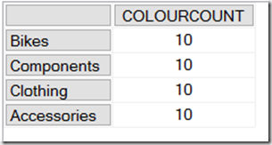
The EXISTING keyword is used within calculations to apply autoexists filtering to a set based on the other hierarchies from the same dimension. The following query contains a calculated measure that counts the number of members on the Color level of the Color hierarchy, and unsurprisingly returns the same value each time it’s called:

WITH
MEMBER MEASURES.COLOURCOUNT AS
COUNT([Product].[Color].[Color].MEMBERS)
SELECT 
{MEASURES.COLOURCOUNT} 
ON 0,
[Product].[Category].[Category].MEMBERS
ON 1
FROM
[Adventure Works]

image

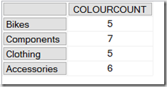
However, if you add the EXISTING keyword just before the set in the calculated measure definition, like so:

WITH
MEMBER MEASURES.COLOURCOUNT AS
COUNT(EXISTING [Product].[Color].[Color].MEMBERS)
SELECT 
{MEASURES.COLOURCOUNT} 
ON 0,
[Product].[Category].[Category].MEMBERS
ON 1
FROM
[Adventure Works]

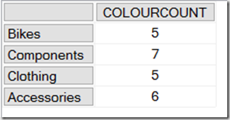
Then you’ll see that the calculation now returns the number of members on the Color level of the Color hierarchy after autoexists filtering has been applied; so for example the first line shows there are five distinct colours associated with the Category Bikes:

image

Summary

OK, after that somewhat lengthy introduction, in part 2 I’ll show you how to use Profiler to monitor what’s going on inside SSAS when you do all of these different types of non empty filtering.


Monitoring SSAS Multidimensional Non Empty Filtering Using Profiler, Part 2

$
0
0

In part 1 of this series I introduced all of the different types of non empty filtering that can occur in Analysis Services and MDX. In this post I’ll show you how you can monitor each of these types of non empty filtering using Profiler using the queries from part 1 as examples.

Profiler events

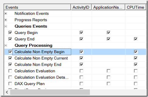
The three Profiler events we’re going to be most concerned with here are:

  • Calculate Non Empty Begin, which is raised when the engine starts a non empty filter
  • Calculate Non Empty Current, which will be raised one or more times when the non empty filter is in progress and which will give us more detail about what’s happening
  • Calculated Non Empty End, which is raised when the engine finishes evaluating a non empty filter

I’ve also included the Query Begin/End events in my traces just to show when query execution starts and finishes. All the queries in this post will be run on a warm cache; although the values used for non empty filtering can be cached, SSAS can’t cache the output of a non empty filter (unless you do something like this) so for our purposes whether the cache is warm or cold is irrelevant.

image

NON EMPTY and NONEMPTY()

In the simplest cases SSAS treats the NON EMPTY statement and the NONEMPTY() function the same, so let’s look again at the following query from my previous post:

SELECT 
{[Measures].[Internet Order Quantity]} 
ON 0,
NON EMPTY
[Product].[Category].[Category].MEMBERS
ON 1
FROM
[Adventure Works]

image

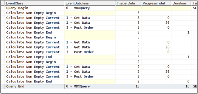
Here’s what our Profiler trace shows us when this query is run:

image

There are several things to notice here:

  • The Duration column tells us how long, in ms, both the query took to run (on the Query End line) and the non empty filter took to evaluate (on the Calculate Non Empty End line).
  • The EventSubclass column, for the Calculate Non Empty Current events, shows the different stages of evaluation. The possible values here are:
    • 1 – cell values are evaluated for the filtering
    • 2 – calculated members are evaluated (this is no longer used from SSAS 2008 on)
    • 3 – the tuples are rendered in the resultset
  • The IntegerData column shows what type of non empty filtering is taking place. The possible values here are:
    • 1 – All non empty filtering using NON EMPTY and NONEMPTY() using a fast algorithm (as shown in the screenshot above)
    • 2 – EXISTING operations using a fast algorithm.  This is a bit misleading though, because due to an internal bug this event will not fire for most uses of the EXISTING statement but will fire for some operations related to regular autoexists.
    • 3 – Autoexists operations using a fast algorithm
    • 11 – All non empty filtering using NON EMPTY and NONEMPTY() using a slower algorithm, for when complex calculations need to be evaluated
    • 12 – as (2) but with the slower algorithm (theoretically possible but should never occur in practice)
    • 13 – as (3) but with the slower algorithm (again, theoretically possible but should never occur in practice)
  • The ProgressTotal column for the Calculate Non Empty Current (as with the Serialize Results Current event) and EventSubclass 1 should return the number of tuples evaluated for the non empty filter. If the number of tuples is greater than 1000 you’ll see multiple events, one for each 1000 tuples, with the last event showing the overall total. Unfortunately there’s a bug here that means it returns one less than the actual number of tuples evaluated. What’s more, in most cases, the non empty filter operations in the SSAS engine are difficult to match to whatever’s going on in the query, so it’s only really useful as a relative measure of how expensive the operation is.

Putting this all together, for this query we can see that there was one non empty filter operation, it was using the fast NON EMPTY algorithm, the ProgressTotal column shows 3 tuples were returned (ie the three Categories on rows) and it took 1ms.

Autoexists

Now let’s look at the autoexists query from the previous post in this series:

SELECT 
{[Measures].[Internet Order Quantity]} 
ON 0,
[Product].[Category].[Category].MEMBERS
*
[Product].[Color].[Color].MEMBERS
ON 1
FROM
[Adventure Works]

image

Here’s what Profiler shows:

image

Even with what looks like a single autoexists operation there are three sets of Non Empty events here, two of which have IntegerData 3 (for autoexists) and one with IntegerData 2 (for EXISTING which, as noted above, is to be expected here with autoexists). The ProgressTotal column returns 26 for a query that returns 24 rows which I guess is near enough correct to be useful.

EXISTS() And Existing

As you might expect, the EXISTS() function produces a result very similar to a straightforward autoexists. Taking the EXISTS() query from my previous post:

SELECT 
{[Measures].[Internet Order Quantity]} 
ON 0,
EXISTS(
[Product].[Category].[Category].MEMBERS
, {[Product].[Color].&[White]})
ON 1
FROM
[Adventure Works]

image

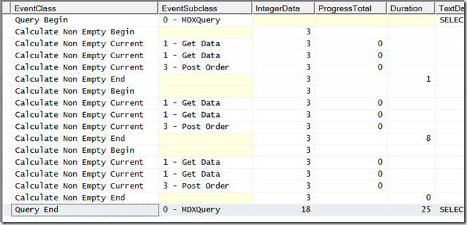
You can see there’s just one Non Empty Begin/End event pair generated, with IntegerData 3, and ProgressTotal returns 0 which means that one tuple is returned:

image

Whereas the use of EXISTING inside a calculated measure, like so:

WITH
MEMBER MEASURES.COLOURCOUNT AS
COUNT(EXISTING [Product].[Color].[Color].MEMBERS)
SELECT 
{MEASURES.COLOURCOUNT} 
ON 0,
[Product].[Category].[Category].MEMBERS
ON 1
FROM
[Adventure Works]

image

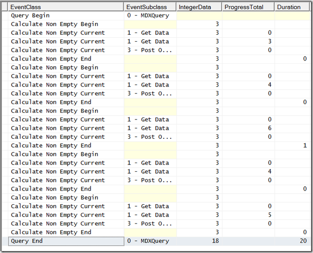
Causes multiple Non Empty Begin/End pairs, very probably one for each member on the hierarchy based on the number of events and the values in the ProgressTotal column (the ProgressTotal values for the second, third, fourth and fifth non empty filters tally with the four values returned by the calculated measure; I don’t know what the first non empty filter is doing) :

image

The WHERE Clause And Subselects

Weirdly enough, the presence of a WHERE clause or a subselect in a query also triggers Non Empty Begin/End events [Subselects are something that a lot of SSAS developers get confused by, especially when it comes to the differences between a subselect and the WHERE clause – I recommend watching this short video if you’re unsure of what they do].

The following query with a WHERE clause generates a single Non Empty Begin/End event pair:

SELECT 
{[Measures].[Internet Order Quantity]} 
ON 0,
[Product].[Color].[Color].MEMBERS
ON 1
FROM
[Adventure Works]
WHERE([Customer].[Total Children].&[5])

image

image

Probably the only value in knowing that this happens is that you can ignore it when you see it.

A query with a subselect instead of a WHERE clause, while it returns exactly the same results in this case, produces different activity in Profiler:

SELECT 
{[Measures].[Internet Order Quantity]} 
ON 0,
[Product].[Color].[Color].MEMBERS
ON 1
FROM
(SELECT {[Customer].[Total Children].&[5]} ON 0
FROM
[Adventure Works])

image

image

Again, if you have a subselect in your query (they are very common in MDX generated by SSRS and Excel) you should ignore this activity. In both cases you’ll note that the IntegerData column shows 3 for autoexists and ProgressTotal shows 0.

Summary

What’s clear from these examples is that trying to relate what’s going on in the query to what you see in Profiler is quite tricky even for seemingly simple queries; for most real-world queries it would be almost impossible to do so with total confidence. That said, when I’m tuning queries I usually comment out large parts of the code to try to isolate problems, thus creating much simpler queries, and I hope the value of this post will lie in you being able to spot similar patterns in Profiler to the ones I show here when you do the same thing. In part 3 of this series I’ll show you some practical examples of how all this information can help you tune your own queries.


New SSAS, Power BI And SQL Server Training Courses For 2016

$
0
0

I’ve just added a number of new 2016 training course dates to the Technitrain site. If you’re looking for Power BI, Analysis Services, SQL Server or Data Science training in London then please check them out! Also, if you’d like to sign up for the Technitrain newsletter to stay up-to-date with our news you can do so here.

Here are more details on the new courses:

SQL Server Performance Tuning and Internals Boot Camp, Bradley Ball, 15-19 February 2016, London
This 5-day hands-on course is designed to provide DBAs with the tools and knowledge that are required to keep their SQL Servers running efficiently and reliably.
http://technitrain.com/coursedetail.php?c=60&trackingcode=CWB

Introduction To Power BI, Chris Webb, 22-23 February 2016, London
A two-day introduction to Microsoft’s exciting new BI tool suitable for BI professionals, analysts, report developers or anyone interested in using it to build reports or dashboards.
http://technitrain.com/coursedetail.php?c=65&trackingcode=CWB
 
Real World Cube Design And Performance Tuning With SSAS Multidimensional,  Chris Webb, 11-13 April 2016, London
A course aimed at intermediate-to-experienced Analysis Services Multidimensional developers, looking at more advanced cube design topics and query performance tuning.
http://technitrain.com/coursedetail.php?c=66&trackingcode=CWB

Mastering DAX, Marco Russo, 20-22 June 2016, London
A three-day introduction to the DAX language used by Power BI, Analysis Services Tabular models and Power Pivot.
http://technitrain.com/coursedetail.php?c=63&trackingcode=CWB

Optimising DAX, Marco Russo, 23-24 June 2016, London
An advanced two-day course for experienced DAX developers who wish to learn how to optimise DAX calculations and queries for performance.
http://technitrain.com/coursedetail.php?c=64&trackingcode=CWB

Introduction to MDX, Chris Webb, 4-6 July 2016, London
A three day course designed for those with little or no experience of MDX, this course will teach you how to write MDX queries and calculations for Analysis Services.
http://technitrain.com/coursedetail.php?c=67&trackingcode=CWB
 
Practical Data Science with Cortana Analytics, Rafal Lukawiecki, 24-27 October 2016, London
This course is aimed at analysts, analytical power users, predictive developers, BI power users and developers, budding data scientists and consultants.
http://technitrain.com/coursedetail.php?c=68&trackingcode=CWB


Two New Books: “The Definitive Guide To DAX” And “’M’ Is For Data Monkey”

$
0
0

I’m not going to pretend that this blog post is a properly impartial review – I know the authors of both of these books to varying degrees – but I thought it was worth writing a few words on two new books I’ve acquired recently which are worth additions to any Power BI enthusiast’s bookshelf or e-reader.

The Definitive Guide To DAX

Something I’ll never understand about my friends Marco Russo and Alberto Russo is their love of writing books – they generally have a new one out every year, sometimes two (personally I find writing books painful). Their latest publication is “The Definitive Guide To DAX” and it does indeed live up to its title. No-one outside the dev team comes close to Marco and Alberto’s knowledge of DAX, the language of Power Pivot, Power BI Desktop modelling and SSAS Tabular, and in this book they have documented everything that they know about it down to the smallest detail. Want to know what the KeepFilters() function does? Or the GenerateAll() function? How about all the new DAX functions and features in the latest versions of Power BI Desktop which will also appear in SSAS 2016 Tabular? They’re all here, and more. As such this is essential purchase for anyone doing serious work on the Microsoft BI platform, although probably more as a reference than a book to read end-to-end. It’s fair to say there’s a certain amount of overlap between this and some of their previous books on Power Pivot and SSAS Tabular, but the language – and the community’s understanding of it – has evolved sufficiently to justify buying this book too.

[I received a free copy of this book for review]

Buy it here from Amazon UK | US

‘M’ Is For Data Monkey

As the author of the only other book on Power Query, I suppose I should really be keeping quiet about “’M’ Is For Data Monkey” in case you buy it instead of mine. However 18 months of UI changes and functionality improvements mean my book is now a bit out-of-date, and what’s more important is that Ken Puls and Miguel Escobar have had the advantage of a lot of real-world experience with Power Query that I didn’t have (indeed no-one had) when I was writing in early 2014. The book itself is not a formal introduction to the M language but a guide to what you can do with it in Power Query; while a lot of what’s here will be useful in Power BI this is definitely a Power Query book and the target audience is Excel Pros rather than BI Pros. The decision to focus on Excel Pros was a good one to make, in my opinion, because it plays to the authors’ strengths and means that the book has a very practical focus. A lot of the tips and tricks here are ones I’ve used successfully myself, and I don’t mind admitting that I learned one or two things from this book as well.

Buy it here from Amazon UK | US

Other Books Are Available…

There are a couple of other new books out that, although I haven’t seen them, will also be worth checking out. Rob Collie has just released Power Pivot and Power BI, essentially the second edition of DAX Formulas For Power Pivot; Matt Allington has just released Learn To Write DAX; both are going to be good choices for Excel users wanting a DAX tutorial. Finally, last week Teo Lachev announced on his blog that he has published the world’s first dedicated Power BI book. Teo is another author whose books I admire so I’m sure it will be excellent, although I’ll be interested to see how he handles the problem of writing about a product that changes so much so quickly.


Monitoring SSAS Multidimensional MDX Query Results Serialisation, Part 1

$
0
0

Profiler (or indeed XEvents) can tell you a lot of interesting things about what happens when SSAS Multidimensional serialises the resultset returned by an MDX query. To be honest, this isn’t something I’ve looked at in detail before but recently I decided to do some research in this area – it turns out that monitoring the Profiler events related to serialisation can be very useful when you’re trying to understand what a Profiler trace is telling you about query execution as a whole.

To start off, let’s look at some very simple examples. Consider the following MDX query on the Adventure Works DW database:

SELECT
{[Measures].[Internet Order Quantity],
[Measures].[Internet Sales Count]}
ON 0,
[Date].[Calendar Year].[Calendar Year].MEMBERS
ON 1
FROM
[Adventure Works]

If you run it in SQL Server Management Studio in an MDX query window, you’ll get the following cellset back:

image

Running a Profiler trace using, amongst others, the Serialize Results Begin, Serialize Results Current and Serialize Results End events shows how SSAS is constructing the cellset returned:

image

The Serialize Results Begin event marks the point where SSAS starts to construct the cellset returned. The Serialize Results Current events that immediately follow it, with EventSubclass “1 – Serialize Axes” show SSAS serialising the tuples that are present on the Columns axis (listed as Axis 0 in the TextData column), the Rows axis (Axis 1) and the Where clause (Slicer Axis). The numeric values in the ProgressTotal column for the Serialize Results Current events shows the number of tuples on each axis: the two tuples on columns are the two measures, the six tuples on rows are the six years, and there’s one tuple on the slicer. After that SSAS gets the data for each of the cell values (as shown by the Query Subcube Verbose event – note that this query is running on a warm cache) and there is then a Serialize Results Current event with EventSubclass “2 – Serialize Cells”; the ProgressTotal column shows that twelve cells (2 columns * 6 rows) in total were returned.  The Serialize Results End event shows that SSAS has finished constructing the cellset and not surprisingly it’s followed immediately by the Query Cube End and Query End events.

Sometimes SSAS needs to do a bit more work to find out what tuples are on an axis before serialisation can begin. The following query adds a NON EMPTY to the rows axis of the query above, so that only the rows that have values are returned:

SELECT
{[Measures].[Internet Order Quantity],
[Measures].[Internet Sales Count]}
ON 0,
NON EMPTY
[Date].[Calendar Year].[Calendar Year].MEMBERS
ON 1
FROM
[Adventure Works]

image

In order to know which years will appear on rows it has to query the cube to find out which ones have values for the measures on columns; as a result the Profiler trace shows a Query Subcube Verbose event appearing now before Serialize Results Begin:

image

This trace deliberately doesn’t show any of events related to the NON EMPTY operation (something I’ll be writing about in future blog posts), but it looks like SSAS can work out which years have values and get the values needed for the cellset back in a single operation so there’s no need for another Query Subcube Verbose event before the Serialize Cells event. Note that now the empty rows have been excluded, the ProgressTotal shows that only four tuples are returned on rows and eight cells are returned overall.

Cellsets are not the only type of resultset that SSAS can return though. Some client tools, most notably Reporting Services, return a tabular dataset that doesn’t have the concept of axes; running the previous query in SSRS gives the following in Profiler:

image

As you can there is now only one Serialize Results Current event and it has the EventSubclass “3 – Serialize SQL Rowset” (even though this is still an MDX query); the ProgressTotal column shows four, which is the number of rows returned.

In Part 2, I’ll look at what happens when a query returns a much larger amount of data.


Monitoring SSAS Multidimensional MDX Query Results Serialisation, Part 2

$
0
0

In part 1 of this series I looked at the basics of monitoring SSAS Multidimensional query resultset serialisation in Profiler. In this post, I’ll be taking a look at what happens for queries that return large amounts of data

Consider the following query on the Adventure Works DW database, which, when I run it in SQL Server Management Studio returns a cellset with 60391 rows:

SELECT
{[Measures].[Internet Order Quantity],
[Measures].[Internet Sales Count]}
ON 0,
NON EMPTY
[Date].[Date].[Date].MEMBERS
*
[Customer].[Customer].[Customer].MEMBERS
*
[Product].[Product].[Product].MEMBERS
ON 1
FROM
[Adventure Works]

image

There are a couple of interesting things to note about this query. First, SQL Server Management Studio on my laptop says that it takes nine seconds to run, even on a warm cache; the Duration column for the Query End event in Profiler, however, shows a value of around six seconds. The three second difference must be the time it takes for SSAS to return the cellset to SQL Server Management Studio, and for SQL Server Management Studio to render the results (my guess is that it’s the second operation that takes the majority of this time – other client tools may be more efficient at rendering large resultsets).

Secondly, in Profiler, you’ll see a much larger number of Serialize Results Current events. In situations where an axis contains more than a thousand tuples, or a cellset contains more than a thousand cells, you’ll see one Serialize Results Current event for each thousand tuples or cells. The ProgressTotal column will show values incrementing by one thousand up to the total number of tuples or cells. So, here’s some of what Profiler shows for the serialisation of the Rows axis:

image

…and here’s the end of the trace, showing the end of the serialisation of the cells (60391 rows * 2 columns = 120782 cells):

image

The third thing to notice is that there is only one Storage Engine operation – shown by the Query Subcube Verbose event in the first Profiler screenshot above – and that hits the Storage Engine cache and is so quick the Duration column shows 0 ms. Getting the raw data isn’t the problem here, and there aren’t any MDX calculations either – which means that it’s the Non Empty filter and construction of the cellset that is taking all the time. Since neither of these operations can be cached (although you can play tricks like this), this explains why the query always takes six seconds to run, even on a warm cache. Further investigation reveals that the Non Empty filter in fact only takes about a quarter of a second, so it’s the construction of a large cellset that’s the real problem here. This is why I say you should always avoid queries that return large amounts of data! SSAS is not very good at returning large resultsets.

Incidentally, don’t fall into the trap of thinking that the values shown in the Duration column for the Serialize Results End event only represents the amount of time taken to construct the cellset. It shows the amount of time since the Serialize Results Begin event, and in between the Begin and End events all kinds of other things necessary for the query to return (such as the evaluation of MDX calculations) could be going on. In a lot of cases the Serialize Results End event shows a duration that is almost the same as the duration for the whole query, but that only means that serialisation was able to start soon after the query began. In order to find the overhead of serialisation you need to work out how long all these other things take and subtract that from the duration shown for Serialize Results End, and that’s easier said than done.

Finally, what can you do to improve performance? Well, in the first post in this series I showed there was a tabular alternative to a cellset, and this is certainly a lot more efficient at returning large amounts of data (although you probably won’t have a choice in this unless you are building your own client tool, and, SSRS uses the tabular format anyway). For this query a tabular resultset is almost two seconds faster to return than a cellset, at just over four seconds:

image

There’s another important technique you can use, once that I have already mentioned in a blog post a couple of years ago but which is worth mentioning again: each cell returned by this query returns a large number of properties that you may not need, and these extra properties have a significant effect on the size of the resultset. Adding a CELL PROPERTIES clause to the query so that you only return the value property, like so:

SELECT
{[Measures].[Internet Order Quantity],
[Measures].[Internet Sales Count]}
ON 0,
NON EMPTY
[Date].[Date].[Date].MEMBERS
*
[Customer].[Customer].[Customer].MEMBERS
*
[Product].[Product].[Product].MEMBERS
ON 1
FROM
[Adventure Works]
CELL PROPERTIES VALUE

…takes another two seconds off the duration of the query, whether you use a tabular resultset or a cellset:

image


Disabling Excel PivotTable Grouping And Session Cubes In SSAS Multidimensional

$
0
0

The Excel PivotTable grouping functionality that is available when you are connected to an SSAS Multidimensional cube (but not a Tabular model) is a Very Bad Thing indeed. In my experience it is a major cause of query performance problems – not just for the person running the query, but because it is so resource intensive for everyone else trying to query the cube too. This post from a few years ago gives some more details about why custom grouping, and the CREATE SESSION CUBE MDX statements that it uses behind the scenes, are so expensive.

Up until now it was impossible to prevent users from using custom grouping but in a recent cumulative update this changed. First of all, I encourage you to read the details of the fix because you will probably want to install the relevant CU for security reasons anyway:

https://support.microsoft.com/en-us/kb/3080856

[And if you are wondering whether you should be installing CUs I strongly suggest you read this post by Aaron Bertrand]

Once the CU has been installed the following new property is added to the msmdrv.ini file:

\OLAP\Query\SessionCubesMode

This will be set to 1. Setting this property to 0 will prevent users from creating session cubes and therefore prevent them from using Excel’s custom grouping functionality.

My opinion is that it’s a good idea to disable session cubes and custom grouping even if you don’t know whether your users are using these features. Yes, your users will lose some functionality and some reports might even break, but you will also save yourself and your users a lot of problems. If your users need to do custom grouping in a report that is usually an indication that you have missed something in your dimension design, and that an extra attribute hierarchy or two is necessary.

[Thanks to Akshai for this information]


Finding All Selected Items In A Slicer In Excel 2016 Using TextJoin()

$
0
0

When you are using slicers with an Excel PivotTable it’s often useful to be able to get a comma-delimited list of the items selected in that slicer for use in a report title. It’s not easy to do though, and in fact this is one of those topics that lots of people have blogged about over the years: here’s my MDX approach, here’s Erik Svensen’s post on using the new DAX ConcatenateX() function, and there are also posts by Rob Collie like this one. None of these techniques are ideal though: my personal favourite is the ConcatenateX() approach, but that only works with SSAS Tabular 2016 (and then only if you can create a measure on the model) or Power Pivot in Excel 2016, and not at all if you’re using SSAS Multidimensional or earlier versions of SSAS Tabular.

However, after discovering the new TextJoin() function in Excel 2016 the other week I realised that this would provide yet another way to solve this problem. Here’s a simple example using a PivotTable and slicer connected to a Power Pivot model:

image

The highlighted cell F3 showing a comma-delimited list of all the items selected in the slicer has the following Excel formula:

=TEXTJOIN(
    ", ",
    TRUE,
     IFERROR(
      CUBERANKEDMEMBER(
        "ThisWorkbookDataModel",
        Slicer_Product,
        ROW(
         INDIRECT("1:"&CUBESETCOUNT(Slicer_Product))
        )
       ),
      "")
     )

Important: this needs to be entered as an array formula, so instead of hitting Enter after typing in the formula you need to hit Ctrl+Shift+Enter. You’ll see the formula surrounded by braces {} in the formula bar when you do this:

image

image

This formula relies on the fact that the selection in a slicer (in the example above the slicer has the name Slicer_Product) can be treated the same as the output of the Excel CubeSet() function, which means that you can use the CubeSetCount() function to find the number of items selected and the CubeRankedMember() function to get the name of any single item in the selection. It also uses the Row()/Indirect() trick described here to create an array of numbers from 1 to the number of items selected in the slicer, which in turn provides the rank values to pass to the CubeRankedMember() function.

The beauty of this approach is that it works for Power Pivot and all versions of SSAS Tabular and Multidimensional, and doesn’t require any measures to be created on your models/cubes. It even works in Excel Online, so it will work inside Power BI, although it doesn’t seem to be possible to create array formulas in Excel Online yet so you need to create the formula on the desktop before you deploy. Of course you need the latest build of Excel 2016 for all this to work, and at the time of writing most people don’t have Excel 2016 and even if they do they probably won’t have a build (Version 16.0.6568.2025 or higher) with TextJoin() in it yet. But this will be a great solution in the distant future when everyone has Excel 2016, I promise!

You can download the sample Excel 2016 workbook here.

I also have to acknowledge the help of David Hager in writing this formula – we had a conversation about how TextJoin() behaves in array formulas in the comments of my earlier post and in doing so he provided the basic approach for me.


Viewing all 104 articles
Browse latest View live