Quantcast
Channel: Analysis Services - Chris Webb's BI Blog
Viewing all 104 articles
Browse latest View live

SSAS 2016 Locking Improvements

$
0
0

I first became aware of the server-wide lock taken out by SSAS when processing finishes – and the issues that this can cause – from this blog post by Andrew Calvett back in 2009. More information on how locking works in SSAS can be found in chapter 26 of “Microsoft SQL Server 2008 Analysis Services Unleashed”, while the most comprehensive discussion of this topic can be found in this post by Jason Howell:
https://blogs.msdn.microsoft.com/jason_howell/2012/07/03/analysis-services-stops-accepting-new-connections-processing-commit-locks-hurt/

Over the years I’ve worked with several customers who have run into locking problems as a result of users querying while processing or synchronisation are taking place, so as a result I was interested to read the following paragraph in the white paper on “Automated Partition Management For Analysis Services Tabular Models” that was published a few months ago:

Note that commit operations have been optimized considerably for tabular models in SQL Server 2016. This has caused noticeable improvements in locking and blocking for some customers with near-real time processing requirements. Database write-commit locks are required to safely complete tasks such as merging pending changes, persisting files to disk, clearing some cached state, deletion of old files, etc. In previous versions of Analysis Services, a server-level write commit lock was taken while most of these tasks were performed. With SQL Server 2016, the server-level locks are far more limited; they are only taken while producing the delta of transaction updates, and are then immediately released.

This is very good news, and in fact the improvements apply to SSAS Multidimensional 2016 as well as SSAS Tabular 2016. The ever-helpful Akshai Mirchandani of the dev team has given me more details on the changes, so here’s a summary of what happens during a commit operation and what’s new in SSAS 2016:

  • First of all, a database read-commit lock is taken to analyse all the pending changes.
  • Next a database write-commit lock is taken so that the transaction can be committed safely. This is the lock that can be blocked by long-running queries, and this is where the ForceCommitTimeout property comes into play with the result that these long-running queries may get cancelled.
  • This lock is held while the pending changes are merged together.
  • At this point SSAS is ready to do the commit, and where it takes a server-level write-commit lock. This is also the point where the improvements in SSAS 2016 have been made.
    • In previous versions SSAS would update the master.vmp file in place and hold the server-level write-commit lock while that happens and while some other, potentially time-consuming things like clearing cached state and deleting all the old files take place. This could in some cases result in the server-level write-commit lock being held for an extended period.
    • Instead in SSAS 2016 a delta of all the transaction updates are written to a .txn file, and after that the server commit lock is released. The time-consuming tasks mentioned in the previous bullet still take place but after the server-level write-commit lock has been released. This means the server-level write-commit lock is now held for a very short amount of time, and what’s more that amount of time is quite consistent.
  • Finally, all remaining locks such as the database write-commit lock are released.

I haven’t had a chance to test these changes in a production system yet but it sounds like anyone that needs to process or synchronise regularly throughout the day will benefit from upgrading to SSAS 2016.


Power BI, SSAS Multidimensional And Dynamic Format Strings

$
0
0

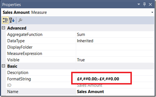
If you’re building reports in Power BI against SSAS Multidimensional cubes then you may have encountered situations where the formatting on your measures disappears. For example, take a very simple SSAS Multidimensional cube with a single measure called Sales Amount whose FormatString property is set in SSDT to display values with a £ sign:

image

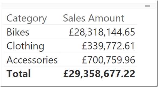
When you build a report using the Table visualisation in Power BI Desktop using this measure, the formatted values are displayed correctly:

image

However, if you add a SCOPE statement to the cube to alter the format string of the measure for certain cells, as in this example which sets the format string for the Sales Amount measure to $ for Bikes:

SCOPE([Measures].[Sales Amount], [Product].[Category].&[1]);
    FORMAT_STRING(THIS)="$0,0.00";
END SCOPE;

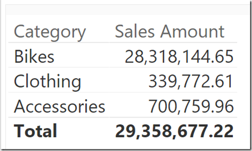
…then you’ll find that Power BI displays no formatting at all for the measure:

image

What’s more (and this is a bit strange) if you look at the DAX queries that are generated by Power BI to get data from the cube, they now request a new column to get the format string for the measure even though that format string isn’t used. Since it increases the amount of data returned by the query much larger, this extra column can have a negative impact on query performance if you’re bringing back large amounts of data.

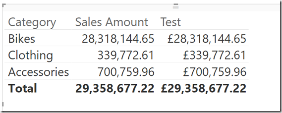
There is no way of avoiding this problem at the moment, unfortunately. If you need to display formatted values in Power BI you will have to create a calculated measure that returns the value of your original measure, set the format string property on that calculated measure appropriately, and use that calculated measure in your Power BI reports instead:

SCOPE([Measures].[Sales Amount], [Product].[Category].&[1]);
    FORMAT_STRING(THIS)="$0,0.00";
END SCOPE;

CREATE MEMBER CURRENTCUBE.[Measures].[Test] AS
[Measures].[Sales Amount],
FORMAT_STRING="£0,0.00";

image

Thanks to Kevin Jourdain for bringing this to my attention and telling me about the workaround, and also to Greg Galloway for confirming the workaround and providing extra details.


SSAS Multidimensional: Are Your Indexes Processed?

$
0
0

If you are using SSAS Multidimensional and you use Process Update to process your dimensions, here’s something for you to try: run a Process Default on your cube. Does it finish in a few seconds? Then you’re ok. If it doesn’t, and it takes minutes or even longer then read on – you might have a problem that’s causing slow query performance.

One of the most common sources of query performance problems I see with my SSAS Multidimensional customers is unprocessed aggregations and indexes. If you run a Process Update on a dimension it may result in indexes and aggregations being dropped from partitions in your cubes; for more details on this, and why it happens, see this post:

https://blog.crossjoin.co.uk/2010/05/12/what-happens-when-you-do-a-process-update-on-a-dimension/

This classic post by Darren Gosbell explains how you can check if you have unprocessed aggregations on a partition:

http://geekswithblogs.net/darrengosbell/archive/2008/12/02/ssas-are-my-aggregations-processed.aspx

However, unprocessed indexes can also be a problem for query performance too. You can tell if the indexes on a partition are built by using the discover_partition_dimension_stat DMV. Here’s an example of how to use it for a partition in the Adventure Works database:

SELECT
DIMENSION_NAME, ATTRIBUTE_NAME, ATTRIBUTE_INDEXED,
ATTRIBUTE_COUNT_MIN, ATTRIBUTE_COUNT_MAX
FROM SystemRestrictSchema($system.discover_partition_dimension_stat
        ,DATABASE_NAME = 'Adventure Works DW 2008'
        ,CUBE_NAME = 'Adventure Works'
        ,MEASURE_GROUP_NAME = 'Internet Sales'
        ,PARTITION_NAME = 'Internet_Sales_2003')


[For some background on running SSAS DMV queries, see here]

Here’s what the above query returns, a list of dimensions and attributes that are related to the partition:

image

If the ATTRIBUTE_INDEXED column shows false then indexes are not built for the attribute on the dimension. In this example no indexes are built at all on the partition; if I do a Process Index or Process Default on this partition, here’s what the DMV returns:

image

Now you can see the ATTRIBUTE_INDEXED property is set to true for most attributes. Note that there is an (All) attribute that is never indexed, and if you have set the AttributeHierarchyEnabled property to false or the AttributeHierarchyOptimizedState property to NotOptimized on an attribute, it will not have indexes built for it either (this is typically done to improve processing performance – see here for a few more details).

In a real-world cube it is likely that only a few indexes will be dropped on partitions as a result of a Process Update on a dimension, and even then this will depend on whether any changes take place in the dimension’s data, so you will have to look down the list of attributes returned by this DMV very carefully to see if ATTRIBUTE_INDEXED returns false when it should be returning true.

The solution to this problem, as several of the posts I’ve linked to above suggest, is to always run a Process Default on your cube as the last step in your processing schedule. A Process Default will process any object that is in an unprocessed state, so it will automatically rebuild any aggregations or indexes that are dropped as a result of Process Updates on dimensions.


Obscure MDX Month: Recreating The Star Ratings Measure In MDX Using Excel Functions

$
0
0

I still love MDX, but I’m aware that I blog about it less and less – which is a shame, I know. Therefore I’ve decided that for the next four weeks I’m going to write about some obscure MDX topics that hopefully will make all you SSAS MD diehards out there feel less neglected… even if they don’t have much practical use.

Let’s start off with recreating my ever-popular DAX star-ratings measure in MDX. Well, not exactly pure MDX, but did you know that in MDX you can call some Excel functions (in the same way you can call some VBA functions)? It’s a really, really bad thing to do from a query performance point of view, but it does allow you to do some useful calculations that might otherwise be impossible. Here’s a query on the Adventure Works cube that uses the Excel Rept() and Unichar() functions (functions that do not exist in MDX proper) to recreate my start-ratings measure:
WITH
MEMBER MEASURES.STARS AS
REPT(
UNICHAR(9733),
CINT([Measures].[Internet Sales Amount]/10000))
+
REPT(
UNICHAR(9734),
10-CINT([Measures].[Internet Sales Amount]/10000))

SELECT {[Measures].[Internet Sales Amount],MEASURES.STARS} ON 0,
ORDER(
[Date].[Date].[Date].MEMBERS,
[Measures].[Internet Sales Amount],
BDESC)
ON 1
FROM
[Adventure Works]


image

Here’s the same measure used in a PivotTable:

image


Obscure MDX Month: Current and CurrentOrdinal

$
0
0

When you are writing an MDX expression, everywhere you use a set you can give that set a name and then reference the name later on. This is known as creating an inline named set, something I have blogged about a few times (see here and here) over the years. When you are iterating over a set using a function like Generate() or Filter(), if you give that set a name you can then use the Current and CurrentOrdinal functions to find out more about the item in the set returned at the current iteration.

Consider the following MDX query on the Adventure Works cube:

SELECT
{[Measures].[Internet Sales Amount]}
ON 0,
{[Customer].[Gender].[Gender].MEMBERS
*
[Customer].[Marital Status].[Marital Status].MEMBERS}
ON 1
FROM
[Adventure Works]

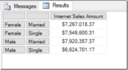
It returns a set of four tuples on rows: every combination of Gender and Marital Status:

image

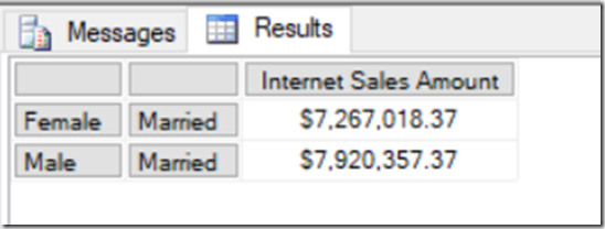
If you pass the set on rows to the Filter() function and give it a name (for example MySet) you can then use the CurrentOrdinal function to find the 1-based ordinal of the current iteration. This query uses the CurrentOrdinal function to filter the set shown above so only the first and third items in the set are returned:

SELECT {[Measures].[Internet Sales Amount]} ON 0,
FILTER(
{[Customer].[Gender].[Gender].MEMBERS
*
[Customer].[Marital Status].[Marital Status].MEMBERS}
AS MYSET,
MYSET.CURRENTORDINAL=1 OR
MYSET.CURRENTORDINAL=3)
ON 1
FROM
[Adventure Works]


image

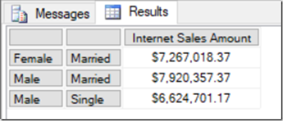
With an inline named set you can also use the Current function to return the tuple at the current iteration. Here’s another query that uses the Current function to remove the tuple (Female, Single) from the set:

SELECT
{[Measures].[Internet Sales Amount]} ON 0,
FILTER(
{[Customer].[Gender].[Gender].MEMBERS
*
[Customer].[Marital Status].[Marital Status].MEMBERS}
AS MYSET,
NOT(
MYSET.CURRENT IS
([Customer].[Gender].&[F],[Customer].[Marital Status].&[S])
)
)
ON 1
FROM
[Adventure Works]

image

I won’t pretend that these functions are massively useful, but fans of super-complex MDX will enjoy this vintage post where I used them.


Obscure MDX Month: Optimising The Performance Of Total-To-Date Calculations In SSAS Multidimensional

$
0
0

Here’s a SSAS Multidimensional MDX tip that I picked up at the PASS Summit back in 2008 at Mosha’s excellent “MDX Deep Dive” precon (incidentally the slides and supporting material are still available here, although a lot of the material is out of date). It’s regarding total-to-date calculations, ie calculations where you are doing a running total from the very first date you have data for up to the current date. The standard way of writing these calculations is something like this:

WITH
MEMBER MEASURES.[TTD Sales] AS
SUM(
NULL:[Date].[Calendar].CURRENTMEMBER,
[Measures].[Internet Sales Amount])

SELECT
[Customer].[Country].[Country].MEMBERS
ON 0,
NON EMPTY
[Date].[Calendar].[Date].MEMBERS
*
[Product].[Product].[Product].MEMBERS
ON 1
FROM
[Adventure Works]
WHERE(MEASURES.[TTD Sales])

This query runs in around 19.2 seconds on my laptop on a cold cache. However if you rewrite it like this:

WITH
MEMBER MEASURES.[PTTD SALES] AS
SUM(
NULL:[Date].[Calendar].CURRENTMEMBER.PARENT.PREVMEMBER,
[Measures].[Internet Sales Amount])

MEMBER MEASURES.[TTD Sales] AS
MEASURES.[PTTD SALES]
+
SUM(
[Date].[Calendar].CURRENTMEMBER.FIRSTSIBLING:
[Date].[Calendar].CURRENTMEMBER,
[Measures].[Internet Sales Amount])

SELECT
[Customer].[Country].[Country].MEMBERS
ON 0,
NON EMPTY
[Date].[Calendar].[Date].MEMBERS
*
[Product].[Product].[Product].MEMBERS
ON 1
FROM
[Adventure Works]
WHERE(MEASURES.[TTD Sales])

…it runs slightly faster: around 16.1 seconds on a cold cache on my laptop. Of course this is a very big query, and on most normal queries the difference in performance would be much less significant, but it could still be useful. In fact it’s very similar to the kind of tricks people used to optimise the performance of YTD calculations back in the days of SSAS 2000 – the subject of my second-ever blog post from December 2004! The idea here is that instead of summing up a large set of dates, the calculation sums up all the dates in the current month and then all the months from the beginning of time up to and including the previous full month. For YTD and most other something-to-date calculations trick like this are no longer needed, and indeed are counter-productive and will make your calculations slower. However it seems that for total-to-date calculations they can still help performance.


Obscure MDX Month: Optimising MDX That Uses The RGB() Function

$
0
0

In the first blog post in this series a few weeks ago I mentioned that calling Excel and VBA functions from MDX came with a query performance penalty. In this post I’ll give you an illustration of this using the VBA function that I suspect is most frequently called in MDX: the RGB() function.

Take the following MDX query as a baseline:

WITH
MEMBER MEASURES.TEST AS
[Measures].[Internet Sales Amount]
SELECT {[Customer].[Country].[Country].MEMBERS} ON 0,
NON EMPTY
[Date].[Date].[Date].MEMBERS
*
[Product].[Product].[Product].MEMBERS
 ON 1
FROM
[Adventure Works]
WHERE(MEASURES.TEST)
CELL PROPERTIES
VALUE,
FORMATTED_VALUE,
BACK_COLOR


It returns Countries on columns and all non empty combinations of Date and Product on rows, and the calculated measure returns the value of the Internet Sales Amount measure:

image 

On a SE engine cache it runs in 2.5 seconds on my laptop. With a BACK_COLOR property added to the calculated measure that uses the RGB() function to return the code for red if the measure value is greater than $5000, query performance is a lot worse: it goes up to 6.5 seconds on a warm SE cache.

WITH
MEMBER MEASURES.TEST AS
[Measures].[Internet Sales Amount]
,BACK_COLOR=
IIF([Measures].[Internet Sales Amount]>5000,
RGB(255,0,0),
RGB(255,255,255))
SELECT {[Customer].[Country].[Country].MEMBERS} ON 0,
NON EMPTY
[Date].[Date].[Date].MEMBERS
*
[Product].[Product].[Product].MEMBERS
 ON 1
FROM
[Adventure Works]
WHERE(MEASURES.TEST)
CELL PROPERTIES VALUE, FORMATTED_VALUE, BACK_COLOR


image

That’s a big increase just to do some cell highlighting! However in this case the RGB() function can only return two possible integer values, so if you replace the RGB() function with the integers it returns, like so:

WITH
MEMBER MEASURES.TEST AS
[Measures].[Internet Sales Amount]
,BACK_COLOR=
IIF([Measures].[Internet Sales Amount]>5000,
255,
16777215)
SELECT {[Customer].[Country].[Country].MEMBERS} ON 0,
NON EMPTY
[Date].[Date].[Date].MEMBERS
*
[Product].[Product].[Product].MEMBERS
 ON 1
FROM
[Adventure Works]
WHERE(MEASURES.TEST)
CELL PROPERTIES VALUE, FORMATTED_VALUE, BACK_COLOR

…then the query returns in around 3.5 seconds. The last thing to remember is that IIF() statements can perform better if one branch returns null, and in this case we can replace the integer value 16777215 that gives the white background with a null and get the same result:

WITH
MEMBER MEASURES.TEST AS
[Measures].[Internet Sales Amount]
,BACK_COLOR=
IIF([Measures].[Internet Sales Amount]>5000,
255,
NULL)
SELECT {[Customer].[Country].[Country].MEMBERS} ON 0,
NON EMPTY
[Date].[Date].[Date].MEMBERS
*
[Product].[Product].[Product].MEMBERS
 ON 1
FROM
[Adventure Works]
WHERE(MEASURES.TEST)
CELL PROPERTIES VALUE, FORMATTED_VALUE, BACK_COLOR

Now the query returns in around 3 seconds, only 0.5 seconds slower than the original with no colour coding.


Obscure MDX Month: Deselecting Members In An Excel PivotTable Leads To Missing Rows

$
0
0

Here’s some interesting (and borderline buggy) Excel PivotTable behaviour I learned about today from Charles-Henri Sauget, as well as the workaround for it courtesy of the great Greg Galloway.

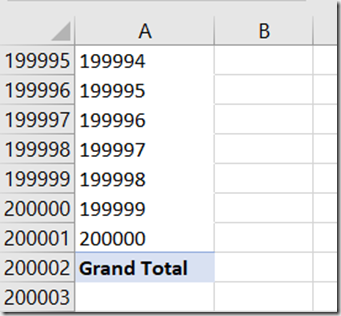
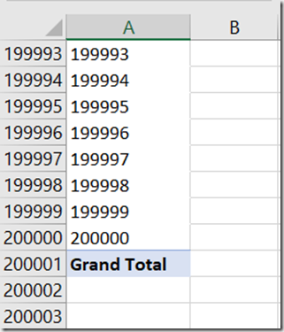
Say you have a large dimension attribute hierarchy with 200,000 members on it in SSAS MD (or the equivalent in Tabular or Power Pivot) and drop it onto the rows of an Excel PivotTable. As you would expect, you get a PivotTable with 200,000 rows in it:

image

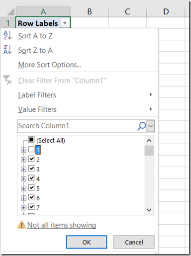
However if you then deselect just one member on rows like so:

image

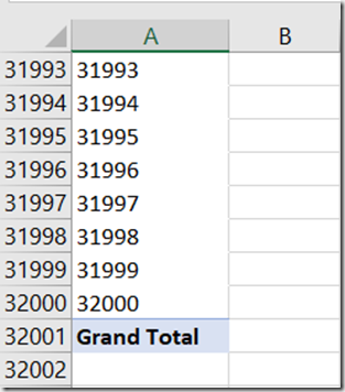
…you’ll find that the PivotTable does not have 199,999 rows – in Excel 2016 it only has 32,000 rows:

image

(different versions of Excel may return different numbers of rows here, but still not the full number).

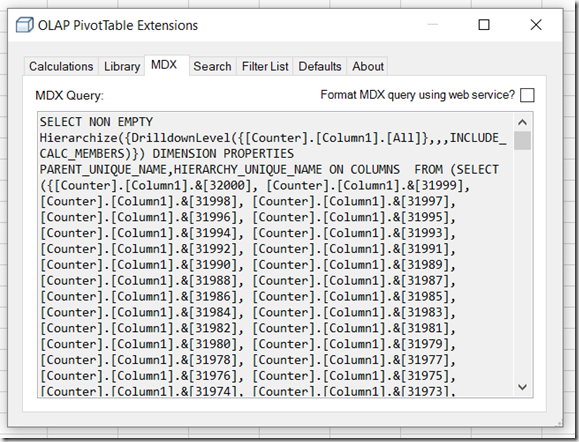
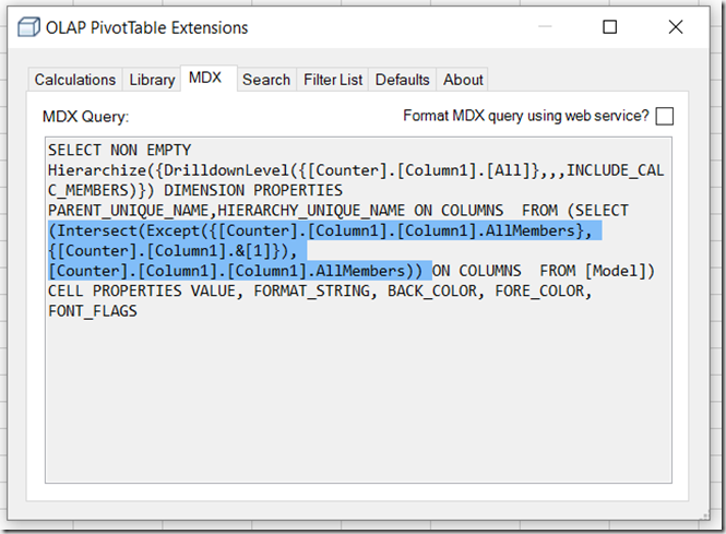
If you look at the MDX generated by Excel it consists of all of the member unique names that are still selected, and unsurprisingly it’s a gigantic query:

image

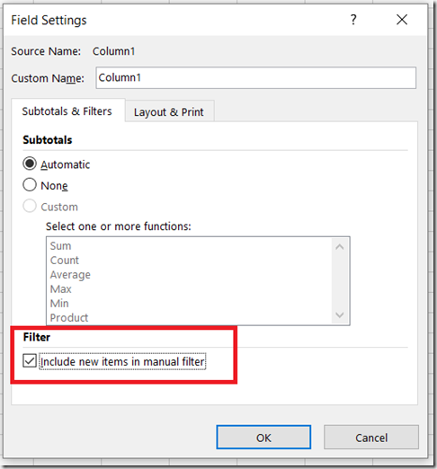
However, it turns out you can make Excel do the sensible thing and use the Except() function to return everything apart from the deselected member by going to the Field Settings dialog and selecting “Include new items in manual filter”:

image

image

This then gives you the expected number of rows in the PivotTable:

image

I suspect the reason Excel is generating the crazy-long MDX statement by default is that it’s the only way to prevent new members being added to the PivotTable if they are added to the attribute hierarchy in future. On a really large attribute hierarchy, though, the risk is that the resulting MDX query might exceed the maximum length of a query, so Excel has to truncate the number of members returned to make the query shorter. With “Include new items in manual filter” selected, though, it’s ok if new members do get added to the PivotTable in the future so it’s ok to use the Except() function in the query.


The Power Query Branding Problem

$
0
0

A few years ago I started blogging about Power Query. Back then life was simple: I put “Power Query” in the title of a post and everyone knew what I was writing about, because Power Query was an Excel add-in you could download and install. Now, however, the technology has been renamed “Get & Transform” in Excel 2016 and is a native feature of Excel; the name “Power Query” only applies to the add-in for Excel 2010 and 2013. What’s more, the same technology is used in Power BI’s Query Editor and it’s also now in Azure Analysis Services, Analysis Services 2017 Tabular and the Common Data Service. This is obviously a good thing – I think Power Query is one of the best things to come out of Microsoft in the last decade – but it also presents me with a problem. How can I write about this technology if it doesn’t have a single, official, easily identifiable name?

In more recent times I’ve written posts with unwieldy names like “Introduction to Insert Topic Name Here in Power Query/Power BI/Excel 2016 Get & Transform” and in the future I suppose this will have to grow to “Introduction to Insert Topic Name Here in Power Query/Power BI/Excel 2016 Get & Transform/Analysis Services Data Loading/Common Data Service”. Tagging and categorising blog posts can help here, I know, but it’s the title of a blog post that’s the main determining factor as to whether it gets read or not when someone is looking at a list of search results. It’s getting ridiculous, but how else can I ensure that someone searching for the solution to a data loading problem in Excel 2016 Get & Transform will find a post I’ve written that contains the answer but shown in Power BI?

Inside Microsoft I understand that the team that builds this technology is known as the Power Query team. I certainly think about this technology as being called Power Query, as do a lot of other people in the community. However, my argument is that I can’t just use the name “Power Query” when I’m writing or speaking about this technology because most of its users – especially those who are new to it and who need the most help – don’t think of it as “Power Query”. They think of it as Excel 2016 Get & Transform, the Query Editor in Power BI Desktop and so on, the specific instances of it.

Maybe I’m making too big a deal of this, but in my opinion this is a problem not just for me but for Microsoft too. We all know how much developers rely on internet searches to find solutions to problems, and not having a single name for this technology makes it much harder to search successfully. This in turn makes it less likely that when a developer runs into a problem they will be able to solve it, which in turn means they are less likely to want to use this technology in future.

What’s the answer? It has to be to make the “Power Query” brand visible somewhere in the UI of all the products that use Power Query technology. I know there’s a risk of confusing users instead of helping them here (am I using Power Query or Power BI?), but it could be as simple as making a few small changes like renaming the “Query Editor” window to be the “Power Query Editor”:

image

I think that would be enough to let people know that “Power Query” is a technology in its own right and that content referring to “Power Query” is relevant to Excel, Power BI, SSAS and everywhere else that Power Query is used. It would also be nice if, now that M is the official name of the M language (and not Power Query Formula Language), the Advanced Editor window and the Custom Column dialog let users know that the code they were writing in them was in a language called M and not some mysterious, nameless scripting language.

What do you think? I’m interested to hear your comments and opinions…

UPDATE: victory is ours! See this comment from Faisal Mohamood of the Power Query team below
Hey there Chris – what you are saying makes complete sense. Power Query is the name of this capability and we will highlight the name of this capability as such in experiences where you are working with Power Query (and M).


Tuning MDX Calculations That Use The Root() Function

$
0
0

Something that I have vaguely known about for years (for example from Mosha’s post here), but somehow never blogged about, is that using the Root() function in MDX calculations is not great for performance. I’m pretty sure that someone once told me that it was intended for use with defining subcubes for SCOPE statements and not inside calculations at all, which maybe why it hasn’t been optimised. Anyway, here’s an example of the problem and how to work around it.

Take the following query on the Adventure Works cube:

WITH
MEMBER MEASURES.DEMO AS
([Measures].[Internet Sales Amount],
ROOT([Date]))

SELECT
{[Measures].[Internet Sales Amount],
MEASURES.DEMO}
ON 0,
NON EMPTY
[Date].[Calendar].[Calendar Year].MEMBERS
*
[Customer].[Customer].[Customer].MEMBERS
ON 1
FROM
[Adventure Works]

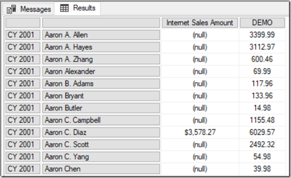
It returns sales for all customers by year, and the calculated measure returns the sales for each customer across all dates using the Root() function.

image

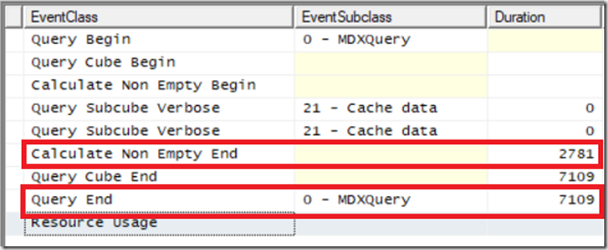
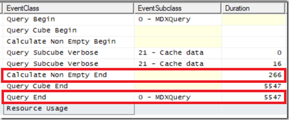
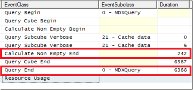
On a warm SE cache (which means the amount of time taken by the query will be dependent on how quickly SSAS can do the calculation and evaluate the Non Empty) on my laptop this takes a touch over 7 seconds:

image

Notice also that the Calculate Non Empty End event tells us that the Non Empty filter alone took 2.8 seconds (see here for some more detail on this event).

Now if you rewrite the query, replacing the Root() function with the All Member on the Calendar hierarchy like so:

WITH
MEMBER MEASURES.DEMO AS
([Measures].[Internet Sales Amount],
[Date].[Calendar].[All Periods])

SELECT
{[Measures].[Internet Sales Amount],
MEASURES.DEMO}
ON 0,
NON EMPTY
[Date].[Calendar].[Calendar Year].MEMBERS
*
[Customer].[Customer].[Customer].MEMBERS
ON 1
FROM
[Adventure Works]

The query returns the same results, but in just over 5.5 seconds and with the Non Empty taking about 10% of the time it previously took.

image

I’m making a big assumption here though: the Root() function in the first query returns a tuple containing every All Member from every hierarchy on the Date dimension, not just the All Member from the Calendar hierarchy, so while these two queries return the same results the calculations are not equivalent. You can still get a performance improvement, though, by replacing the Root() function with the tuple it returns, although the resulting MDX will look very messy.

First, to find what the Root() function returns just use a query like this:

WITH
MEMBER MEASURES.ROOTRETURNS as
TUPLETOSTR(ROOT([Date]))
SELECT {MEASURES.ROOTRETURNS} ON 0
FROM
[Adventure Works]

Run it in SQL Server Management Studio and you can copy/paste the tuple from the query results:

image

Here’s the tuple I get from my (somewhat hacked around) Date dimension:

([Date].[Fiscal].[All Periods],[Date].[Calendar].[All Periods],[Date].[Calendar Weeks].[All Periods],
[Date].[Fiscal Weeks].[All Periods],[Date].[Fiscal Year].[All Periods],[Date].[Date].[All Periods],
[Date].[Calendar Quarter].[All Periods],[Date].[Fiscal Quarter].[All Periods],
[Date].[Calendar Semester].[All Periods],[Date].[Fiscal Semester].[All Periods],
[Date].[Day of Week].[All Periods],[Date].[Day Name].[All Periods],
[Date].[Day of Month].[All Periods],[Date].[Day of Year].[All Periods],
[Date].[Calendar Week].[All Periods],[Date].[Month Name].[All Periods],
[Date].[Calendar Year].[All Periods],[Date].[Fiscal Semester of Year].[All Periods],
[Date].[Calendar Semester of Year].[All Periods],[Date].[Fiscal Quarter of Year].[All Periods],
[Date].[Calendar Quarter of Year].[All Periods],[Date].[Month of Year].[All Periods],
[Date].[Fiscal Week].[All Periods],[Date].[Calendar Week of Year].[All Periods],
[Date].[Fiscal Week of Year].[All Periods],[Date].[Current Date].[All Periods],
[Date].[Is2002].[All Periods],[Date].[Month Day].[All Periods])

Yuck. Anyway, with this gigantic tuple inserted into our calculation like so:

WITH
MEMBER MEASURES.DEMO AS
([Measures].[Internet Sales Amount],
[Date].[Fiscal].[All Periods],[Date].[Calendar].[All Periods],[Date].[Calendar Weeks].[All Periods],[Date].[Fiscal Weeks].[All Periods],[Date].[Fiscal Year].[All Periods],[Date].[Date].[All Periods],[Date].[Calendar Quarter].[All Periods],[Date].[Fiscal Quarter].[All Periods],[Date].[Calendar Semester].[All Periods],[Date].[Fiscal Semester].[All Periods],[Date].[Day of Week].[All Periods],[Date].[Day Name].[All Periods],[Date].[Day of Month].[All Periods],[Date].[Day of Year].[All Periods],[Date].[Calendar Week].[All Periods],[Date].[Month Name].[All Periods],[Date].[Calendar Year].[All Periods],[Date].[Fiscal Semester of Year].[All Periods],[Date].[Calendar Semester of Year].[All Periods],[Date].[Fiscal Quarter of Year].[All Periods],[Date].[Calendar Quarter of Year].[All Periods],[Date].[Month of Year].[All Periods],[Date].[Fiscal Week].[All Periods],[Date].[Calendar Week of Year].[All Periods],[Date].[Fiscal Week of Year].[All Periods],[Date].[Current Date].[All Periods],[Date].[Is2002].[All Periods],[Date].[Month Day].[All Periods])

SELECT
{[Measures].[Internet Sales Amount],
MEASURES.DEMO}
ON 0,
NON EMPTY
[Date].[Calendar].[Calendar Year].MEMBERS
*
[Customer].[Customer].[Customer].MEMBERS
ON 1
FROM
[Adventure Works]

The query is a little slower – just over 6 seconds- but still faster than the first query using Root(), and the Non Empty filter is still fast:

image

Something else to watch out for with Root(), and another good reason not to use it in calculations, is that it returns an error in certain multiselect scenarios as Richard Lees describes here.


SSAS Multidimensional HOLAP Storage: Even More Useless Than You Might Think

$
0
0

In almost 20 years of using Analysis Services I have never, ever used HOLAP storage. However the other week I was with a customer that was using ROLAP storage on top of Exasol and while query performance was generally good, I wondered whether building an aggregation or two in SSAS might help query performance in some cases. Surely HOLAP could be useful here? Sadly not.

What I hadn’t realised was that when you use HOLAP storage and process a partition, SSAS generates exactly the same fact table-level SQL query that is used to process a MOLAP partition. It then uses this data to build any aggregations you have defined and after that throws the data it has read away, leaving only the aggregations stored in MOLAP mode. Therefore you get exactly the same, slow processing performance as pure MOLAP storage and worse query performance! It even executes the SQL query when there are no aggregations defined. I had assumed SSAS would generate one SQL query for each aggregation and get just the summarised data needed by the aggregation but I was wrong. This means that for the kind of scenarios where ROLAP on a fast relational database is becoming more popular (for example when working with large data volumes and/or real-time data) HOLAP is not a viable option.


Creating A Partitioned Table In SSAS Tabular 2017 And SSDT Using M Functions

$
0
0

One of the coolest new features in SSAS Tabular 2017 and Azure Analysis Services is the integration of Power Query and M for data loading. Over the last year or so the Analysis Services team blog has posted a lot of fairly complex examples of how to use this functionality, but now that the latest release of SSDT has proper support for shared expressions I thought it would be a good idea to show a simple example of how to use it to create a partitioned table using M functions.

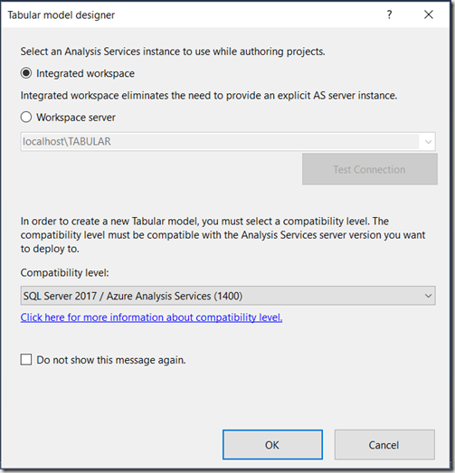
For this example I’ll be using the FactInternetSales fact table from the Adventure Works DW sample database, and the aim is to create a table in an SSAS Tabular project that has one partition for each year of data in FactInternetSales. Assuming that a new SSAS Tabular project has been created at the 1400 compatibility level with an integrated workspace:

image

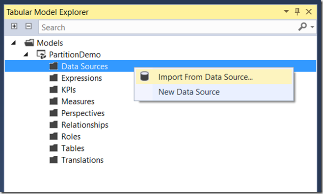
…the first thing to do is to right-click on the Data Sources folder in the Tabular Model Explorer pane and select Import From Data Source:

image

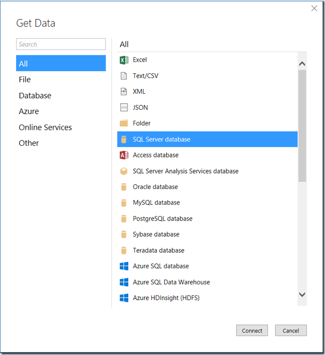
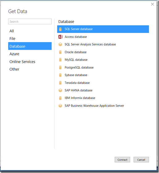
This brings up the Get Data dialog:

image

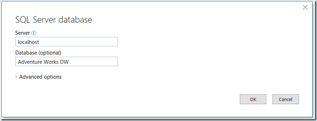
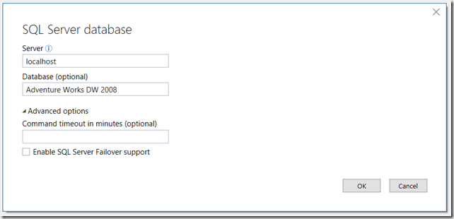
Select SQL Server database and then click Connect. Enter the server name and database name in the SQL Server database dialog:

image

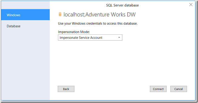
Choose how SSAS is to authenticate when it connects to the SQL Server database and click Connect:

image

Select the FactInternetSales table from the list of tables in the Adventure Works DW database:

image

This opens the Query Editor window; in it there is one query called FactInternetSales:

image

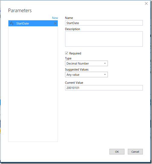
Here’s where it gets interesting. The first thing to do is to create a function that returns a filtered subset of the rows in the FactInternetSales table using the technique I blogged about here for Power BI. On the Query Editor menu bar, click Query/Parameters/New Parameter and create two new parameters called StartDate and EndDate that return the numbers 20010101 and 20011231. Here’s what they should look like:

image

image

These parameters are going to be used to filter the OrderDateKey column on the FactInternetSales table. Do this by clicking on the down arrow on the column header of OrderDateKey then selecting Number Filters and then Between:

image

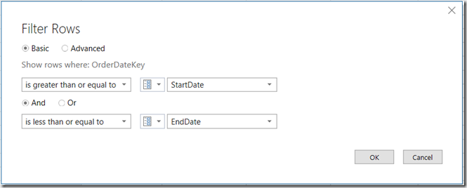
In the Filter Rows dialog use the StartDate parameter for the start of the filter range and the EndDate parameter for the end of the filter range, then click OK:

image

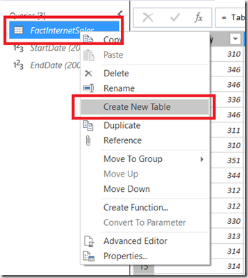
Because the OrderDateKey contains dates stored as numbers in the YYYYMMDD format the result is a table that only contains sales where the order date is in the year 2001. This table should not be loaded into SSAS though, so right click on the FactInternetSales in the Queries pane and make sure that the Create New Table is not checked:

image

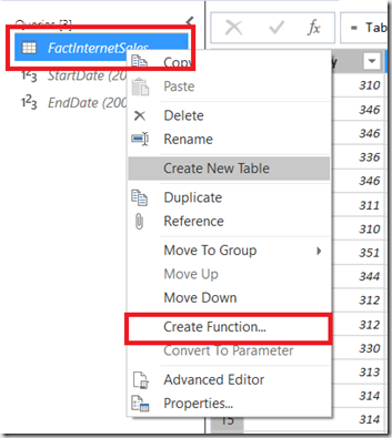
Next, on the same right-click menu, select Create Function:

image

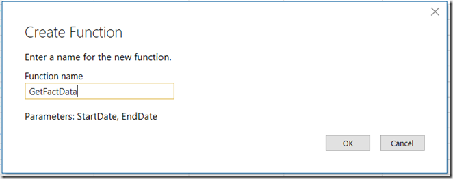
In the Create Function dialog name the new function GetFactData then click OK:

image

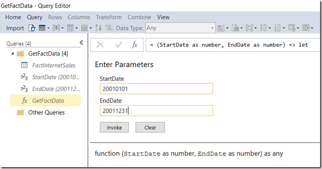
The new GetFactData function will now be visible in the Queries pane; enter 20010101 for the StartDate parameter and 20011231 for the EndDate parameter and click Invoke:

image

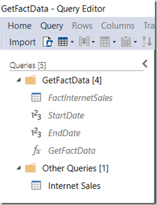
This creates yet another new query called Invoked Function which should be renamed Internet Sales:

image

Right-click on this query and make sure Create New Table is selected. Next, click the Import button on the toolbar to close the Query Editor and load the Internet Sales table into SSAS.

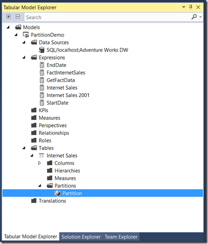
At this point the Tabular Model Explorer will show all of the queries created above listed under the Expressions folder, and a single table called Internet Sales with a single partition:

image

Next, right-click on the Internet Sales table in the Tables folder and select Partitions:

image

This opens the Partition Manager dialog. Rename the existing partition to Internet Sales 2001:

image

Note that the M query for this partition calls the GetFactData() function to get the rows from FactInternetSales where OrderDateKey is between 20010101 and 20011231:

let
    Source = GetFactData(20010101, 20011231)
in
    Source

Click the New button to create new partitions, one for each year of data in the FactInternetSales table. Each new partition will initially contain the same M code shown above and should be edited so that the query gets data for the appropriate year:

image

Click OK, and the end result is a table with one partition per year:

image

What’s the point of using M functions to return the data for a partition, rather than the traditional method of using a SQL query embedded in each partition? One reason to do this would be to make maintenance easier: if you need to do something like add a new column to a fact table, rather than editing lots of partitions you just need to edit the function and all the partitions will reflect that change. I can think of a few others, but I’ll save them for future blog posts…


Drillthrough On Calculated Members In SSAS MD 2017 Using DAX Expressions, Part 1

$
0
0

Without a doubt one of the most useful features of SSAS Tabular 2017 is the new Detail Rows Expression property. It allows you to control exactly which columns and rows appear when you do a drillthrough – something that is particular important when you’re doing a drillthrough on a calculation, and something that SSAS MD users have also wanted to have for a long time now. For example, imagine that you have an Excel PivotTable that is sliced by a single date and a calculated member that shows a year-to-date sum of sales calculation: when a user does a drillthough they would expect to see data for all the fact data that contributes to the value they have clicked on, which in this case means data for all dates from the beginning of the year up to the selected date; this is what the Detail Rows Expression property makes possible and this is exactly what a regular drillthrough in SSAS MD doesn’t do.

There have been many attempts at solving this problem in SSAS MD, from Mosha’s blog post back in 2008 to these custom functions in the Analysis Services Stored Procedure Project (for a few more weeks still on Codeplex, but when Codeplex dies available here on GitHub). None of these solutions have been perfect and all have involved a certain amount of .NET code. In this series of posts I’m going to describe a slightly different approach, and while it isn’t perfect either and is very complex (you’ll need to be good at MDX and DAX to implement it) I think it has a lot to recommend it, not least because no .NET code is required. In this first post I’m going to demonstrate some of the functionality that makes my approach possible; in part 2 I’ll put it all together into a working solution.

First thing to note: you have been able to query SSAS MD using DAX as well as MDX since SQL Server 2012 SP1 CU3. Most client tools, like Excel, generate MDX queries but Power BI for example generates DAX queries when you create a Live connection to SSAS MD. To learn more about DAX support in SSAS MD this video of a session of mine from SQLBits from a few years ago is a good place to start; it’s fairly old but most of the content is still relevant.

This in turn means that you can create a Rowset action (not a Drillthrough action) in SSAS MD that return the results of a DAX query. Here’s an example of an action that does this:

image

The Action Expression property is an MDX expression that returns the text of the query to be executed and whose results will be displayed to the user as the output of the drillthrough. In this case the MDX expression consists of one string, and that string is a DAX query that returns a list of Sales Order Numbers, Line Numbers and their associated Sales Amounts:

EVALUATE
SELECTCOLUMNS(
'Sales Order',
"Sales Order Number",
'Sales Order'[Sales Order Number],
"Sales Order Line Number",
'Sales Order'[Sales Order Line Number],
"Sales Amount",
[Sales Amount])

Here’s the result in Excel:

image

image

This is just a static query though, and for an action you will need to generate a query dynamically to return an appropriate table of data depending on which cell the user has drilled through on.

However before I carry on there’s an important question that needs to be addressed. You may be wondering why I’m using a DAX query for this, when I could be using an MDX DRILLTHROUGH statement (as in the approaches linked to above) or an MDX SELECT statement. The problem with a DRILLTHROUGH statement is that it can only accept an MDX SELECT statement that returns a single cell in its first parameter; this means it’s not possible to get it to return more complex resultsets like the one required for the year-to-date example above. Normal MDX SELECT statements don’t suffer from this restriction and it would indeed be possible to dynamically generate one that meets any need. Unfortunately when the results of an MDX SELECT statement are returned from a Rowset action you have no control over the format of the column headers that are returned, and they are often not pretty at all. A DAX query, in contrast, gives you complete control over the data that is returned and the way the column headers are formatted.

The last question I’m going to address in this post is how the DAX query can be made dynamic. To do this I’m going to use the new DAX IN operator, which is only available in SSAS 2017. As always with DAX, there’s a great article describing it written by Marco Russo here:

https://www.sqlbi.com/articles/the-in-operator-in-dax/

Here’s how the DAX query above can be adapted to return the Sales Orders for just two dates using the IN operator:

EVALUATE
FILTER(
CALCULATETABLE(
SELECTCOLUMNS(
'Sales Order',
"Sales Order Number",
'Sales Order'[Sales Order Number],
"Sales Order Line Number",
'Sales Order'[Sales Order Line Number],
"Sales Amount",
[Sales Amount]),
'Date'[Date.Key0] IN {20030101, 20030102}),
[Sales Amount]>0)

image

In this example, the ‘Date’[Date.Key0] column is the column that contains the key values of the Date attribute on the Date dimension in my SSAS cube. To make this dynamic, you need an MDX expression that will return a query like the one above and, in particular, return a different list of date keys depending on what the user has drilled through on. The MDX GENERATE() function can be used to do this: you can use it to iterate over the set of existing members on the Date attribute of the Date dimension and output a comma-delimited list of key values from each member:

"EVALUATE
FILTER(
CALCULATETABLE(
SELECTCOLUMNS(
'Sales Order',
""Sales Order Number"",
'Sales Order'[Sales Order Number],
""Sales Order Line Number"",
'Sales Order'[Sales Order Line Number],
""Sales Amount"",
[Sales Amount]),
'Date'[Date.Key0] IN {" +
GENERATE(EXISTING [Date].[Date].[Date].MEMBERS,
[Date].[Date].CURRENTMEMBER.PROPERTIES("KEY"), ",")
+ "}),
[Sales Amount]>0)"

If this expression is used in an action and a user drills down on, say, the month April 2003, the following DAX query is generated and run to get all the Sales Orders for all the days in April 2003:

EVALUATE
FILTER(
CALCULATETABLE(
SELECTCOLUMNS(
'Sales Order',
"Sales Order Number",
'Sales Order'[Sales Order Number],
"Sales Order Line Number",
'Sales Order'[Sales Order Line Number],
"Sales Amount", [Sales Amount]),
'Date'[Date.Key0] IN
{20030401,20030402,20030403,20030404,20030405,
20030406,20030407,20030408,20030409,20030410,20030411,
20030412,20030413,20030414,20030415,20030416,20030417,
20030418,20030419,20030420,20030421,20030422,20030423,
20030424,20030425,20030426,20030427,20030428,20030429,
20030430})
, [Sales Amount]>0)

OK, that’s more than enough for one post. In my next post I’m going to look at some of the shortcomings of this approach, how they can be (partly) worked around, and demonstrate a full solution for drillthrough on a regular measure and also on a year-to-date calculation.


Drillthrough On Calculated Members In SSAS MD 2017 Using DAX Expressions, Part 2

$
0
0

If you read part 1 of this series you probably already have a good idea of how I’m going to use DAX queries in actions to implement drillthrough on calculated members. However, there is one last major problem to solve – and no 100% fool-proof way of solving it.

That problem is that there is a maximum length of (as far as I can tell) 32768 characters for the DAX query that is generated by the action. If you exceed that limit you’ll see an error in Excel when you drillthrough:

image

This is the result of the generated DAX query being truncated before Excel tries to run it. As you can imagine, if you have large dimensions and you’re generating a DAX query with thousands of key values in an IN expression, it’s very easy to hit the maximum query length. What can you do to make this less likely?

Probably the most effective method is to check whether the IN clause will contain all of the possible key values on the dimension (most likely because no attributes from the dimension are used in the query), and if so don’t bother including that dimension in the DAX query. Here’s an example of how this can be done:

IIF(
COUNT(EXISTING [Date].[Date].[Date].MEMBERS) =
COUNT([Date].[Date].[Date].MEMBERS),
"",
",'Date'[Date.Key0] IN {
" +
GENERATE(EXISTING [Date].[Date].[Date].MEMBERS ,
[Date].[Date].CURRENTMEMBER.PROPERTIES("KEY"), ",")
+ "}
")

Another option is to use NonEmpty() to remove any members from the drillthrough that have no data, like so:

IIF(
COUNT(EXISTING [Date].[Date].[Date].MEMBERS) =
COUNT([Date].[Date].[Date].MEMBERS),
"",
",'Date'[Date.Key0] IN {
" +
GENERATE(EXISTING
NONEMPTY([Date].[Date].[Date].MEMBERS, [Measures].[Sales Amount])
, [Date].[Date].CURRENTMEMBER.PROPERTIES("KEY"), ",")
+ "}
")

However, if these techniques (and there may be others) still don’t reduce the length of the query to an acceptable length you will want to try to fail as gracefully as possible and show a more helpful error message than the one above. You can do this with the DAX Error() function, like so:

IIF(
COUNT(EXISTING [Customer].[Customer].[Customer].MEMBERS) =
COUNT([Customer].[Customer].[Customer].MEMBERS),
"",
",'Customer'[Customer.Key0] IN {
" +
IIF(COUNT(
{EXISTING
NONEMPTY(
[Customer].[Customer].[Customer].MEMBERS,
[Measures].[Sales Amount])}
AS CustomerList)>7000,
"ERROR(
""Please reduce your selection on the Customer dimension
 or remove it from your PivotTable"")",
GENERATE(
CustomerList
, [Customer].[Customer].CURRENTMEMBER.PROPERTIES("KEY"), ",")
)
+ "}
")

In this example, if the resulting DAX IN expression for the Customer dimension will have more than 7000 keys in it, the entire DAX query returns a custom error message instead:

image

Once again this is a far from perfect solution – I would have liked to test the total number of characters in the query, but if you do that you have to write the expression twice, once in the first parameter of IIF() and once in one of the results, and that would be horrible. My gut feeling is that you should only use this technique on dimensions with a large number of members on the key attribute.

Putting this all together, for a simple cube based on data from Adventure Works with three dimensions (Date, Product and Customer) here’s what a complete Action Expression for a regular measure might look like:

"EVALUATE
FILTER(
CALCULATETABLE(
SELECTCOLUMNS(
'Sales Order',
""Sales Order Number"",
'Sales Order'[Sales Order Number],
""Sales Order Line Number"",
'Sales Order'[Sales Order Line Number],
""Sales Amount"",
[Sales Amount])
" +
IIF(
COUNT(EXISTING [Date].[Date].[Date].MEMBERS) =
COUNT([Date].[Date].[Date].MEMBERS),
"",
",'Date'[Date.Key0] IN {
" +
GENERATE(EXISTING
NONEMPTY([Date].[Date].[Date].MEMBERS,
[Measures].[Sales Amount])
, [Date].[Date].CURRENTMEMBER.PROPERTIES("KEY"), ",")
+ "}
") +
IIF(
COUNT(EXISTING [Customer].[Customer].[Customer].MEMBERS) =
COUNT([Customer].[Customer].[Customer].MEMBERS),
"",
",'Customer'[Customer.Key0] IN {
" +
IIF(
COUNT(
{EXISTING NONEMPTY([Customer].[Customer].[Customer].MEMBERS,
[Measures].[Sales Amount])} AS CustomerList)>7000,
"ERROR(""Please reduce your selection on the Customer dimension
or remove it from your PivotTable"")",
GENERATE(
CustomerList
, [Customer].[Customer].CURRENTMEMBER.PROPERTIES("KEY"), ",")
)
+ "}
") +
IIF(
COUNT(EXISTING [Product].[Product].[Product].MEMBERS) =
COUNT([Product].[Product].[Product].MEMBERS),
"",
",'Product'[Product.Key0] IN {
" +
GENERATE(EXISTING
NONEMPTY([Product].[Product].[Product].MEMBERS,
[Measures].[Sales Amount])
, [Product].[Product].CURRENTMEMBER.PROPERTIES("KEY"), ",")
+ "}
") +
"),
[Sales Amount]>0)"


What about a calculated measure though? Assuming that  you have a time utility/date tool/shell dimension, you can use a Condition expression on the action above to make sure it only gets executed for the member on the time utility dimension that contains the non-calculated values, in this case called [Actual Value]:

([Measures].CURRENTMEMBER IS [Measures].[Sales Amount]) AND
([Date Calculations].[Date Calculations].CURRENTMEMBER IS
[Date Calculations].[Date Calculations].&[Actual Value])

image

Now, let’s say there is a calculated member on the time utility dimension that contains a year-to-date calculation with the following definition:

CREATE MEMBER
CURRENTCUBE.[Date Calculations].[Date Calculations].[Year-To-Date]
AS
AGGREGATE(
PERIODSTODATE(
[Date].[Calendar].[Year],
[Date].[Calendar].CURRENTMEMBER),
[Date Calculations].[Date Calculations].&[Actual Value]);

You can create a new action that has a Condition expression as follows that restricts it to the year-to-date calculation:

([Measures].CURRENTMEMBER IS [Measures].[Sales Amount]) AND
([Date Calculations].[Date Calculations].CURRENTMEMBER IS
[Date Calculations].[Date Calculations].[Year-To-Date])

Now, the final problem to solve is to generate a DAX query that returns all of the Sales Orders from the beginning of the current year up to and including the selected date – the Sales Orders that a user would expect to see when they drilled through on the year-to-date calculated member above.

Here’s a modified MDX expression for the Date dimension that returns a DAX expression that finds all of the dates associated with the current selection on the Date dimension, finds the maximum date, then filters the drillthrough DAX query by all dates from the beginning of the current calendar year up to and including the maximum date:

IIF(
COUNT(EXISTING [Date].[Date].[Date].MEMBERS) =
COUNT([Date].[Date].[Date].MEMBERS),
"",
", VAR FilteredDates = FILTER('Date', 'Date'[Date.Key0] IN {
" +
GENERATE(
EXISTING
NONEMPTY([Date].[Date].[Date].MEMBERS,[Measures].[Sales Amount]) ,
[Date].[Date].CURRENTMEMBER.PROPERTIES("KEY"), ",")
+ "})
VAR MaxDate = MAXX(FilteredDates, 'Date'[Date.Key0])
VAR MaxYear = MAXX(FilteredDates, 'Date'[Year])
RETURN
FILTER('Date', 'Date'[Date.Key0]<=MaxDate && 'Date'[Year]=MaxYear)
")

Here’s the complete MDX expression for the year-to-date drillthrough:

"EVALUATE
FILTER(
CALCULATETABLE(
SELECTCOLUMNS(
'Sales Order',
""Sales Order Number"",
'Sales Order'[Sales Order Number],
""Sales Order Line Number"",
'Sales Order'[Sales Order Line Number],
""Sales Amount"",
[Sales Amount])
" +
IIF(
COUNT(EXISTING [Date].[Date].[Date].MEMBERS) =
COUNT([Date].[Date].[Date].MEMBERS),
"",
", VAR FilteredDates = FILTER('Date', 'Date'[Date.Key0] IN {
" +
GENERATE(
EXISTING
NONEMPTY([Date].[Date].[Date].MEMBERS,[Measures].[Sales Amount]) ,
[Date].[Date].CURRENTMEMBER.PROPERTIES("KEY"), ",")
+ "})
VAR MaxDate = MAXX(FilteredDates, 'Date'[Date.Key0])
VAR MaxYear = MAXX(FilteredDates, 'Date'[Year])
RETURN
FILTER('Date', 'Date'[Date.Key0]<=MaxDate && 'Date'[Year]=MaxYear)
") +
IIF(
COUNT(EXISTING [Customer].[Customer].[Customer].MEMBERS) =
COUNT([Customer].[Customer].[Customer].MEMBERS),
"",
",'Customer'[Customer.Key0] IN {
" +
IIF(COUNT({
EXISTING
NONEMPTY([Customer].[Customer].[Customer].MEMBERS,
[Measures].[Sales Amount])} AS CustomerList)>7000,
"ERROR(""Please reduce your selection on the Customer dimension or
remove it from your PivotTable"")",
GENERATE(
CustomerList
, [Customer].[Customer].CURRENTMEMBER.PROPERTIES("KEY"), ",")
)
+ "}
") +
IIF(
COUNT(EXISTING [Product].[Product].[Product].MEMBERS) =
COUNT([Product].[Product].[Product].MEMBERS),
"",
",'Product'[Product.Key0] IN {
" +
GENERATE(EXISTING
NONEMPTY([Product].[Product].[Product].MEMBERS,
[Measures].[Sales Amount])
, [Product].[Product].CURRENTMEMBER.PROPERTIES("KEY"), ",")
+ "}
") +
"),
[Sales Amount]>0)"

I warned you it was going to be complicated, didn’t I? You can download a SSAS MD 2017 .abf backup file containing the sample database and the two actions here.


The Biml Book, And Some Thoughts On Biml And SSAS

$
0
0

I know what you’re thinking: why is Chris blogging about a book on Biml when he’s not remotely interested in SSIS? Well, you’re right, SSIS isn’t my thing (though as an SSAS developer it’s important to keep up-to-date on the tools that the SSIS people on your team use) and yes, as you may have guessed, I got a freebie review copy because I’m an Apress author and I’m friends with one of the authors, Andy Leonard. There is, though, a good reason why I want to learn about Biml: you can use it to generate SSAS databases as well as SSIS packages.

First of all, the book itself. “The Biml Book” is a new book written by a team of Biml experts that teaches you pretty much everything you need to know about Biml. I’m always a bit worried by books with a large number of authors because I know how difficult it is to maintain a consistent style, but in this case I couldn’t see any joins. As someone with no previous experience of Biml. I found the book very clear, concise and easy to read. I highly recommend it as an introduction to the topic.

Of course the chapter on using Biml with SSAS was the most interesting for me. The main reason why SSAS people aren’t as excited about Biml as SSIS people are is that we just don’t usually have the same amount of boring, repetitive work that begs to be automated, and we already have AMO and TOM when we do need to automate the creation of SSAS objects. Indeed, I’ve only ever met one person who is using Biml with SSAS. So when would you use Biml and SSAS? The book provides a good, honest answer:

Biml can be a great fit for Analysis Services use cases, but there are some exceptions.

Just as with SSIS, one of the great advantages of Biml is that it easily allows scale-out architectures through automation. This makes it a good choice when it comes to multi-tenancy and/or multi-server environments.

Given the ability to automate structures and deployments through metadata, Biml frameworks can also include cube projects that can be driven with some of the same metadata that was used to build data integration frameworks.

Conversely, SSAS Multidimensional/Tabular can require the specification of additional types of metadata to automate its creation. After all, cubes and tabular models are largely just metadata containers on top of relational structures. If you want to use your own metadata to drive the creation of bespoke SSAS projects that could support any SSAS feature, you essentially need to duplicate the entire SSAS feature set in your metadata store. This will result in complex models that may be very difficult and time-consuming to maintain, potentially leading to longer instead of shorter development and deployment times. In a nutshell, Biml isn’t for all SSAS projects, but for the pattern-heavy, scale-out projects where it does fit, it’s tremendously valuable.

I’ll give you an example of where I think Biml and SSAS make a good match. I’ve worked with several companies who do what I call B2B BI: they create, host and manage Microsoft BI solutions for their customers. They have a standard template solution that connects to a particular type of data source (for example, their customers’ Dynamics databases), builds a data warehouse and then puts SSAS and maybe some reports on top. As a result they end up with multiple copies of the same solution, with the only difference being that each copy contains a different customer’s data – a classic example of a “multi-tenancy and/or multi-server environment” as described in the extract above. This style of BI will become more and more common in the future because cloud-based services like Azure SSAS and Power BI (both now support Azure AD B2B) make it much easier to implement, and I think Biml could play a very important role here: you don’t want to build and manage hundreds of near-identical SSAS databases, and their supporting ETL, manually.


Using the Resource Usage Profiler Event For SSAS Multidimensional Query Performance Tuning, Part 1: Rows Scanned And Rows Returned

$
0
0

If you’re performance tuning SSAS Multidimensional Storage Engine issues, the Resource Usage Profiler event can provide a lot of useful information about what’s going on behind the scenes when you run a query. This is something I have blogged about in the past (and it will be useful to read this post before carrying on) but recently I’ve done some more research into this area and found out a lot more things about what this event tells you.

For my testing I created a very simple cube from a single fact table. The table contained 5000 rows and two columns: a dimension key column containing the values 1 to 5000, and a measure column that always contained the value 1. From this I built a single measure group with a single measure called My Measure, and a single dimension built from the dimension key column with 5000 members on it called ID.

Consider the following MDX query:

SELECT 
{[Measures].[My Measure]}
ON 0
FROM
[MyCube]
WHERE([ID].[ID].&[1])

Here’s the output:

image

In this query the WHERE clause filters the output to one member from the ID dimension, which in turn returns data from one row in the underlying fact table, and so My Measure returns 1. If the query is run on cold cache, the Resource Usage Profiler event returns the following:

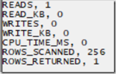
image

The ROWS_RETURNED value here returns 1, which is what you might expect – the query results show data from one row in the underlying fact table. The ROWS_SCANNED value is 256 though. Why? Chapter 20 of the book “Microsoft SQL Server 2008 Analysis Services Unleashed” has a lot of detail about how SSAS MD stores data on disk, but the important point here is that the data in a partition is stored on disk in segments, with each segment made up of pages, and when a query is run SSAS will scan all the pages that it thinks contain data. The ever-reliable Akshai Mirchandani of the SSAS dev team helped me with the remaining information I needed:

  • There are 65536 rows of data per segment
  • There are 256 pages per segment
  • There are therefore, at most, 256 rows per page

So in this case ROWS_SCANNED shows 256 because one complete page was scanned.

Modifying the query to slice on two members from ID like so:

SELECT 
{[Measures].[My Measure]}
ON 0
FROM
[MyCube]
WHERE([ID].[ID].&[1]:[ID].[ID].&[2])

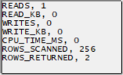
image

…results in a ROWS_RETURNED of 2 and a ROWS_SCANNED that is still 256, because the two rows must be stored in the same page:

image

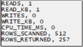
…while asking for 257 members from ID in the WHERE clause like so:

SELECT 
{[Measures].[My Measure]}
ON 0
FROM
[MyCube]
WHERE([ID].[ID].&[1]:[ID].[ID].&[257])

Results in a ROWS_RETURNED of 257 and a ROWS_SCANNED of 257 – obviously 2 pages are now being scanned to get the data needed for the query.

image

Finally, the query:

SELECT 
{[Measures].[My Measure]}
ON 0
FROM
[MyCube]
WHERE([ID].[ID].&[5000])

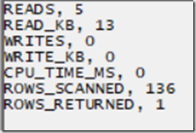
…returns a rows scanned of 136:

image

This must be because the final page, which doesn’t contain the full 256 rows, is scanned. 5000-136=4864, and 4864/256=19, so there must be 20 pages of data: 19 pages of 256 rows and one final page of 136 rows.

I don’t think it’s worth getting too hung up on the exact values that ROWS_SCANNED and ROWS_RETURNED, especially given that they return totals for all Storage Engine activity for all measure groups for the whole query, but knowing that they tell you roughly how much work is being done my the Storage Engine means that you can use them to watch for warning signs that something isn’t working properly when you’re performance tuning queries. In subsequent parts of this series I’ll show some practical examples of this.

Using the Resource Usage Profiler Event For SSAS Multidimensional Query Performance Tuning, Part 2: Many-To-Many Relationships And Non-Materialised Referenced Relationships

$
0
0

You probably know that using many-to-many relationships or non-materialised referenced relationships can be bad for Analysis Services Multidimensional query performance. How can you measure their impact, though? In the first post in this series I showed how the Resource Usage Profiler event could be used to to monitor Storage Engine activity; in this post I’ll use it to show the effect of using these features on the amount of Storage Engine activity that takes place during query execution.

Many-to-many relationships

In my previous post I built a very simple SSAS cube with one measure group called Fact from a table with 5000 rows, then built a dimension called ID from that same table with 5000 members on its only hierarchy. For this post I added a second measure group called Fact Bridge based on the same table, added a new role-playing copy of the existing dimension called M2M ID, and then created a many-to-many relationship from this new dimension to the original measure group via the new measure group.

image

Because all the dimensions and measure groups are built from the same table, one member on the M2M ID dimension is linked to just one member on the ID dimension, so selecting a member on the M2M ID dimension will give the same result as selecting the member with the same key on the ID dimension. Even though SSAS see a many-to-many relationship, in the data it’s a one-to-one relationship.

As I showed in my last post, selecting one member from the ID dimension in a query like the following:

select 
{[Measures].[My Measure]} 
on 0,
{[ID].[ID].&[1]}
on 1
from
[M2M Test]

image

…results in a single page of 256 rows being read and a single row being returned from the cube, as shown by the Resource Usage event in a Profiler trace:

image

If the query is changed to use the M2M ID dimension instead:

select 
{[Measures].[My Measure]} 
on 0,
{[M2M ID].[ID].&[1]}
on 1
from
[M2M Test]

image

…the same result is returned, because the member [M2M ID].[ID].&[1] is associated with one member from the [ID].[ID] hierarchy, the member [ID].[ID].&[1], via the intermediate measure group. However the Resource Usage event shows something very different:

image

The ROWS_SCANNED value has gone from 256 to 5256, and ROWS_RETURNED has gone from 1 to 5003! Why? Part of the explanation is that we now have two measure groups that must be scanned, and the Resource Usage statistics are totals for all Storage Engine activity across all measure groups. In this query the Fact Bridge measure group is scanned first to resolve the many-to-many relationship between the M2M ID and ID dimensions, and then the Fact measure group is scanned to get the value for the measure My Measure. The Fact Bridge measure group only accounts for 256 rows scanned and 1 row returned though, the remaining 5000 rows scanned are from the main Fact measure group. The problem here is that SSAS does not translate the filter on the M2M ID dimension into a filter on the ID dimension (this is a limitation of the way SSAS handles many-to-many) so all the rows on the main Fact measure group get scanned in this query.

This explains something that I have blogged about before here, namely that if you partition your measure group by a dimension that is used in a many-to-many relationship you’ll see that all partitions are scanned and not just the partitions you expect to be scanned. The Resource Usage event shows that even when you don’t see unexpected partition scans happening, using a many-to-many relationship in a query can result in a lot of extra Storage Engine activity and therefore potentially worse query performance.

Non-materialised referenced relationships

Something similar happens when you use non-materialised referenced relationships (although materialised referenced relationships are OK). To test this I created another variation on my original cube, with just one measure group and the ID dimension as before but now with a new, role-playing instance of the ID dimension joining to the measure group through the ID dimension using a non-materialised referenced relationship.

image

image

The following query returns the same result as the two queries above:

select {[Measures].[My Measure]} on 0,
{[Ref ID].[ID].&[1]}
on 1
from
[RefDimTest]

image

…but again, the Resource Usage event shows the entire measure group is being scanned when this query runs:

image

I’m not much of a fan of referenced relationships anyway – you can usually get rid of them by redesigning your SSAS dimensions or your underlying dimensional model – so this one more reason not to use them.

Using the Resource Usage Profiler Event For SSAS Multidimensional Query Performance Tuning, Part 3: Aggregations And Indexes

$
0
0

Building aggregations in your SSAS Multidimensional will make your queries faster, right? While that’s true, they will only make a noticeable difference to performance if your query has Storage Engine-related problems rather than Formula Engine-related problems. What’s more, even when do you have Storage Engine-related problems there are some cases where you may find that aggregations don’t give you the kind of performance boost that you expect. In this post I’ll explain why this can happen, how you can use the Resource Usage Profiler event (as described in parts 1 and 2 of this series) to find out when this is happening, and how you can deal with the problem.

Aggregations make queries go faster for two reasons:

  1. Most importantly they contain pre-aggregated data. For example your fact table might contain data at the Day granularity but an aggregation might contain fact data aggregated up to the Year granularity. This means that when a query needs to get data at the Year granularity, SSAS does not need to read the fact table-level data stored in the partition, it can read the data it needs direct from the aggregation without needing to aggregate any data at query time.
  2. Secondly, because the size of an aggregation is usually a lot smaller than the size of the fact table-level data stored in a partition, it is much faster to read data from an aggregation.

However, regarding this second point, there’s a catch: you’ll know if you’ve read the previous posts in this series that SSAS builds indexes on fact data so it can scan that data very quickly, but most builds of SSAS do not build indexes on aggregations. I say ‘most’ because there were a few builds of SSAS that did build indexes on aggregations, but as this article explains this feature was turned off soon after it was introduced because it was found that the time spent building those aggregations was not usually worth any gain in query performance that resulted.

The Resource Usage Profiler event can be used to monitor the number of rows read and rows scanned when SSAS reads data from an aggregation.Taking the original test query and cube from the previous posts in this series:

SELECT 
{[Measures].[My Measure]}
ON 0
FROM
[MyCube]
WHERE([ID].[ID].&[1])

…the Resource Usage event shows that when run on a cold cache and no aggregations are built on the cube, SSAS scans 256 out of 5000 fact rows of data – a single page – and returns one row:

image

However if this cube has an aggregation built on the ID attribute of the ID dimension, the same granularity as the fact table:

image

…when the query runs and SSAS reads data from this aggregation rather than the fact data, the Resource Usage event returns the following:

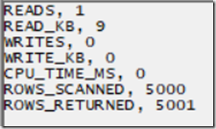
image

Notice that the ROWS_SCANNED value is now 5000. This is because the aggregation has no indexes built on it so SSAS has to scan all the rows in the aggregation. Reading data from an aggregation at the same granularity as the fact data is therefore a lot less efficient than reading data from the original fact data.

Of course, since most aggregations are usually much smaller than the original fact data, the lack of indexes is not so important because scanning all the data is going to be very quick anyway. However, on very large cubes you may need to build some very large aggregations and find that even when your queries hit these aggregations, performance is still bad because of this lack of indexes. If you see this happening, and can see the ROWS_SCANNED value in the Resource Usage event reporting very high values, then it might be a good idea to enable the building of indexes on aggregations.

You can do this by changing the values of the AggIndexBuildEnabled and AggIndexBuildThreshold server properties in the msmdsrv.ini file. Setting AggIndexBuildEnabled to 1 allows SSAS to build indexes on aggregations. It’s not necessary to build indexes on all aggregations though: you can specify that only aggregations larger than a certain number of rows have indexes built using the AggIndexBuildThreshold property. The only public documentation for these properties is given in two articles here and here, and I strongly recommend you read these articles so that you understand the implications of doing this on your processing times. You should only consider changing these properties if you are a very experienced SSAS developer and you monitor the effects carefully – I’m not even sure if changing these properties is supported by Microsoft.

Using Your Own SQL Queries For Tables With Modern Data Sources In SSAS 2016+ And Azure Analysis Services

$
0
0

While the integration of the Power Query engine into Analysis Services Tabular 2017 and Azure Analysis Services with modern data sources will certainly bring a lot of benefits, I think it’s fair to say that the implementation has not been entirely painless. One problem is that it is no longer obvious how to specify your own SQL query to populate a table or partition in your Tabular model – and while the Query Editor is great, there are a lot of cases where this is necessary. In this post I’ll show you how to do this.

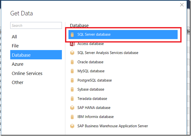
If you’re used to using the Power Query UI in Excel or Power BI Desktop, you’ll notice that when you connect to a SQL Server database using the SQL Server connector in SSDT:

image

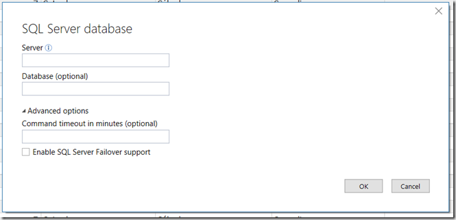
…there is no option to enter your own SQL query when you do so:

image

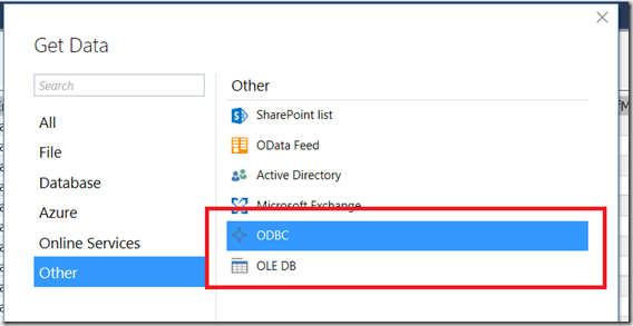
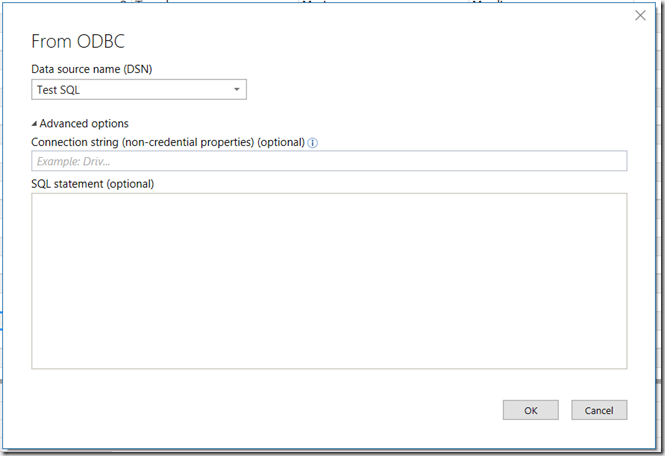
This is deliberate. In Analysis Services, unlike Power BI and Excel, there is a distinction made between data sources and other M queries that return data from those data sources, one that makes a lot of sense in my opinion. While it is possible to enter your own SQL for other data source types, such as OLE DB connections, a data source object is really intended just to define a connection to a data source and not to define what data you want from that data source.

[You may also notice that there’s a “SQL statement” property on a SQL Server data source visible in the Visual Studio properties pane, but I don’t recommend you use it – it doesn’t seem to work well with the rest of the SSDT/Power Query UI]

To import a table or view in your database all you have to do is right-click on your data source and choose Import New Tables; my blog post from September last year describes how to do this, and how to use M functions for creating partitions.

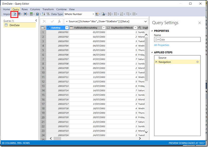
To use your own SQL queries though you need to write some M code. First, import a table – any table, but preferably a small one – and get to the Query Editor UI. In this case I’ve imported the DimDate table from the Adventure Works DW database:

image

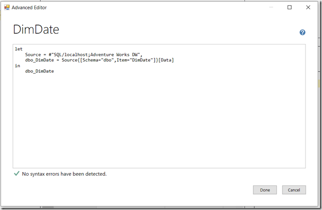
Next, select your query in the Queries pane on the left-hand side of the screen and open the Advanced Editor either by clicking on the relevant button in the toolbar (shown above) or by right-clicking on the query name in the Queries pane. You’ll see the following dialog:

image

The M code will be something like this:

let
    Source = #"SQL/localhost;Adventure Works DW",
    dbo_DimDate = Source{[Schema="dbo",Item="DimDate"]}[Data]
in
    dbo_DimDate

In this example the Source step creates a reference to the data source you have already created, and the dbo_DimDate step gets the contents of the DimDate table from this data source.

You can modify this code to use your own SQL by using the Value.NativeQuery() function (which I have blogged about here):

let
    Source = #"SQL/localhost;Adventure Works DW",
    MyQuery = 
	Value.NativeQuery(
		#"SQL/localhost;Adventure Works DW",
		"SELECT DISTINCT FiscalYear FROM DimDate"
	)
in
    MyQuery

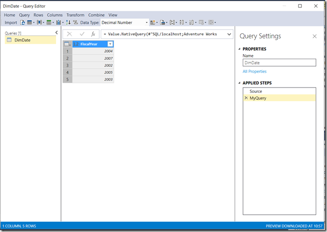
Here what I’ve done is replaced the dbo_DimDate step in the previous query with a step called MyQuery that uses Value.NativeQuery() to run my own SQL.

image

Now all you need to do is click Import and you have the output of the query loaded into SSAS. It would be nice if there was UI support for using your own SQL queries when importing data in the future. Note that, as soon as you use this method, any other steps or queries further downstream will not be able to perform query folding, so you should make sure that you do as much of your filtering and transformation in the SQL as possible otherwise you may encounter performance problems.

The documentation describes a similar – but not identical – workflow for achieving the same result here. Personally I think it’s counter-intuitive that you should click on Expressions to create a Table object! Expressions are used for functions and other M code that is shared by the M queries used by Tables.

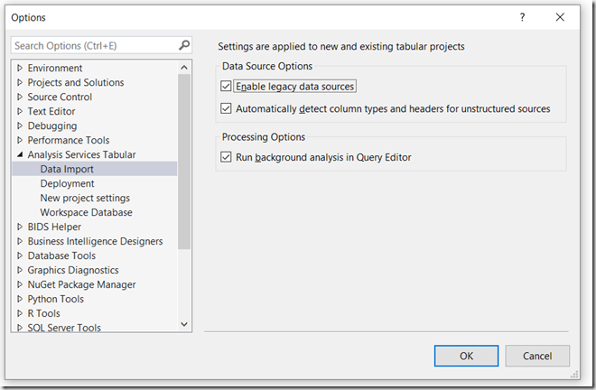
An alternative to doing all this is to go back to the old way of doing things and use a legacy data source rather a modern data source in SSDT. You lose the ability to use the Query Editor and M if you do this, but in a lot of cases you probably won’t care. The 17.4 release of SSDT for Visual Studio 2015, released in December 2017, has exposed a property that allows you to create legacy data sources again easily. In Visual Studio, go to the Tools menu and select Options and in the Options dialog go Analysis Services Tabular/Data Import and check “Enable legacy data sources”:

image

When you do this, you’ll notice two new options when you right-click on Data Sources in the Tabular Model Explorer pane: Import From Data Source (Legacy) and Existing Connections (Legacy).

image

This gives you access to the Table Import wizard that was available in previous versions of Analysis Services Tabular, which not only allows you to enter your own SQL but also creates a legacy data source that in turn makes it easy to use your own SQL when creating partitions.

Setting SQL Server Connection String Properties In Power BI and SSAS Tabular Modern Data Sources

$
0
0

It may not be immediately obvious, but you cannot set your own connection string properties when connecting to SQL Server using the built-in SQL Server connector from either Power BI or a modern data source in Azure SSAS/SSAS Tabular 2017:

image

All you can do is configure the options that are available in the UI, which in the current version of SSDT looks like this:

image

…and which are documented in the Sql.Databases() M function here.

It turns out that the restriction on using your own connection string properties in the built-in SQL Server connector is a deliberate design decision on the part of the Power Query team because, behind the scenes, they use different providers in different circumstances to optimise performance, and because allowing arbitrary connection string properties might make maintaining backwards compatibility difficult in the future.

While your average Power BI user is unlikely to even notice this, for SSAS Tabular developers it could be a big problem: complete control over the connection string is often necessary in enterprise BI scenarios. What are the alternatives then? Well you can use the OLE DB and ODBC connectors instead:

image

Both of these connectors do allow you to set your own connection string properties. For example here’s the UI for a new ODBC connection in SSDT:

image 

The documentation for the Odbc.DataSource and OleDb.DataSource M functions has more detail on how these connectors can be used and how connection string properties can be set. Remember also that the OLE DB Provider for SQL Server was un-deprecated in October 2017.

However, apart from possible performance differences between the two (which you should test yourself – Henk van der Valk wrote a good post on this for SSAS MD and most of what he said is relevant for Tabular) there’s one less-than-obvious difference between these two options: the OLE DB connector does not appear to support query folding right now whereas the ODBC connector does. Of course this isn’t an issue if you’re writing your own SQL queries to import data, but if you do want to use M functions for partitioning (as I show here) you’re likely to get very poor performance with the OLE DB connector.

Viewing all 104 articles
Browse latest View live