Last week a new, free tool for analysing the performance of MDX queries on SSAS Multidimensional was released: Analysis Services Query Analyzer. You can get all the details and download it here:

https://ssasqueryanalyzer.github.io/

…and here’s a post on LinkedIn by one of the authors, Francesco De Chirico, explaining why he decided to build it:

https://www.linkedin.com/pulse/asqa-10-released-francesco-de-chirico/

I’ve played around with it a bit and I’m very impressed – it’s a really sophisticated and powerful tool, and one I’m going to spend some time learning because I’m sure it will be very useful to me. It’s an AddIn for SQL Server Management Studio and captures Profiler and Perfmon data for an MDX query when you run it, does so for a cold and warm cache, and then displays the results in a variety of graphs and charts. And it even has an MDX formatter built in!

You can find a full list of features here, and when you download the tool it comes with very detailed documentation. Definitely a must-have for all serious SSAS Multidimensional developers.

The first mistake that all new Analysis Services Tabular developers make is this one: they create a new project in SSDT, they connect to their source database, they select the tables they want to work with, they click Import, and they then realise that trying to load a fact table with several million rows of data into their Workspace Database (whether that’s a separate Workspace Database instance or an Integrated Workspace) is not a good idea when they either end up waiting for several hours or SSDT crashes because it has run out of memory. You of course need to filter your data down to a manageable size before you start developing in SSDT. Traditionally, this has been done at the database level, for example using views, but modern data sources in SSAS 2017 and Azure Analysis Services allow for a new approach using M.

Here’s a simple example of how to do this using the Adventure Works DW database. Imagine you are developing a Tabular model and you have just connected to the relational database, clicked on the FactInternetSales table and clicked Edit to open the Query Editor window before importing. You’ll see something like this:

…that’s to say there’ll be a single query visible in the Query Editor with the same name as your source table. The M code visible in the Advanced Editor will be something like this:

let
    Source = 
	#"SQL/localhost;Adventure Works DW",
    dbo_FactInternetSales = 
	Source{[Schema="dbo",Item="FactInternetSales"]}[Data]
in
    dbo_FactInternetSales

At this point the query is importing all of the data from this table, but the aim here is to:

1. Filter the data down to a much smaller number of rows for the Workspace Database
2. Load all the data in the table after the database has been deployed to the development server

To do this, stay in the Query Editor and create a new Parameter by going to the menu at the top of the Query Editor and clicking Query/Parameters/New Parameter, and creating a new parameter called FilterRows of type Decimal Number with a Current Value of 10:

The parameter will now show up as a new query in the Queries pane on the left of the screen:

Note that at the time of writing there is a bug in the Query Editor in SSDT that means that when you create a parameter, close the Query Editor, then reopen it, the parameter is no longer recognised as a parameter – it is shown as a regular query that returns a single value with some metadata attached. Hopefully this will be fixed soon but it it’s not a massive problem for this approach.

Anyway, with the parameter created you can now use the number that it returns to filter the rows in your table. You could, for example, decide to implement the following logic:

• If the parameter returns 0, load all the data in the table
• If the parameter returns a value larger than 0, interpret that as the number of rows to import from the table

Here’s the updated M code from the FactInternetSales query above to show how to do this:

let
    Source = 
	#"SQL/localhost;Adventure Works DW",
    dbo_FactInternetSales = 
	Source{[Schema="dbo",Item="FactInternetSales"]}[Data],
    FilterLogic = 
	if 
		FilterRows<=0 
	then 
		dbo_FactInternetSales 
	else 
		Table.FirstN(dbo_FactInternetSales, FilterRows)
in
    FilterLogic 

The FactInternetSales query will now return just 10 rows because the FilterRows parameter returns the value of 10:

And yes, query folding does take place for this query.

You now have a filtered subset of rows for development purposes, so you can click the Import button and carry on with your development as usual. Only 10 rows of data will be imported into the Workspace Database:

What happens when you need to deploy to development though?

First, edit the FilterRows parameter so that it returns the value 0. To do this, in the Tabular Model Explorer window, right-click on the Expressions folder (parameters are classed as Expressions, ie queries whose output is not loaded into Analysis Services) and select Edit Expressions:

Once the bug I mentioned above has been fixed it should be easy to edit the value that the parameter returns in the Manage Parameters pane; for now you need to open the Advanced Editor window by clicking the button shown below on the toolbar, and then edit the value in the M code directly:

Then close the Advanced Editor and click Import. Nothing will happen now – the data for FactInternetSales stays filtered until you manually trigger a refresh in SSDT – and you can deploy to your development server as usual. When you do this, all of the data will be loaded from the source table into your development database:

At this point you should go back to the Query Editor and edit the FilterRows parameter so that it returns its original value, so that you don’t accidentally load the full dataset next time you process the data in your Workspace Database.

It would be a pain to have to change the parameter value every time you wanted to deploy, however, and luckily you don’t have to do this if you use BISM Normalizer – a free tool that all serious SSAS Tabular developers should have installed. One of its many features is the ability to do partial deployments, and if you create a new Tabular Model Comparison (see here for detailed instructions on how to do this) it will show the differences between the project and the version of the database on your development server. One of the differences it will pick up is the difference between the value of the parameter in the project and on in the development database, and you can opt to Skip updating the parameter value when you do a deployment from BISM Normalizer:

CSV files are one of the most commonly used data sources in Power BI and Power Query/Get&Transform, and yet the documentation for the Csv.Document M function is very limited and in some cases incorrect. In this rather long post I’ll show you as many of the capabilities of this useful function as I’ve been able to discover.

The Source parameter

The Csv.Document function returns a table, and the first (and only non-optional) parameter of this function is the source data in CSV format. Normally this is a binary value returned by the File.Contents function. For example take the this simple CSV file with no column headers and one row of data:

The following M code uses File.Contents to read the contents of the file, and then passes the contents to Csv.Document to be interpreted as a CSV file:

let
    Source = File.Contents("C:\CSVTests\SourceFile.csv"),
    ToCSV = Csv.Document(Source)
in
    ToCSV

The output is this:

However it is also possible to pass text to the first parameter of Csv.Document too, for example:

let
    SourceText = "February,Oranges,2",
    ToCSV = Csv.Document(SourceText)
in
    ToCSV

The output of this query is:

In both of these examples I’m relying on the default behaviour of the Csv.Document function with regard to delimiters and other properties, which I’ll explain in more detail below.

Using a record in the second parameter

The second parameter of Csv.Document can be used in several different ways. In code generated by the Query Editor UI it usually takes the form of a record, and the different fields in the record specify how the function behaves in different scenarios. For example, if you connect to the CSV file shown above by selecting the Text/CSV source in the Query Editor UI, you’ll see the following window appear showing a preview of the data and three options:

This results in the following M query:

let
    Source = 
	Csv.Document(
		File.Contents("C:\CSVTests\SourceFile.csv"),
		[
		 Delimiter=",", 
		 Columns=3, 
		 Encoding=1252, 
		 QuoteStyle=QuoteStyle.None
		]),
    #"Changed Type" = 
		Table.TransformColumnTypes(
			Source,
			{
			{"Column1", type text}, 
			{"Column2", type text}, 
			{"Column3", Int64.Type}
			})
in
    #"Changed Type"

The query above shows the Csv.Document function with a record in its second parameter containing four fields: Delimiter, Columns, Encoding and QuoteStyle. There is also a fifth field that can be added to the record, CsvStyle, but this cannot be set anywhere in the UI.

The Data Type Detection option shown in the screenshot gives you three options for detecting the data types in each column of your file: by default it looks at the first 200 rows in the dataset, but you can also ask it to look at the entire dataset (which may be slower) or not to detect data types at all, in which case it will treat all columns as text. In this case data types are not set in the Csv.Document function but in the #”Changed Type” step with the Table.TransformColumnTypes function, but as we will see later it is possible to set column names and data types in a single step with Csv.Document instead.

The Encoding field

The File Origin dropdown menu shown above corresponds to the Encoding field in the Csv.Document function. This integer value specifies the code page used to encode the contents of the file:

In the M query in the previous section the 1252 code page is set explicitly. The following M query sets the (incorrect) 1200 code page for the CSV file shown above:

let
    Source = File.Contents("C:\CSVTests\SourceFile.csv"),
    ToCSV = Csv.Document(Source,[Encoding=1200])
in
    ToCSV

…with the following result:

The Delimiter field

The Delimiter dropdown allows you to specify the delimiter used to separate the columns in each row of data. There are a number of options available through the UI, including commas and tabs, and the Custom option allows you to enter your own delimiter:

If you specify a single character delimiter at this point then the Delimiter field of the record in the second parameter of Csv.Document is set; the Custom and Fixed Width options shown here use a different form of the Csv.Document function described below. If the Delimiter record is not set then a comma is used as the delimiter. If you want to use a special character like a tab then you need to use an M escape sequence; for example to use a tab character as delimiter you need to use the text “#(tab)” which returns a text value containing just a single tab character.

For example, the following query:

let
    Source = "123a456a789",
    ToCSV = Csv.Document(Source, [Delimiter="a"])
in
    ToCSV

Returns:

And this query:

let
    Source = "789#(tab)456#(tab)123",
    ToCSV = Csv.Document(Source, [Delimiter="#(tab)"])
in
    ToCSV

Returns:

The Columns field

The Columns field specifies the number of columns in the table returned by Csv.Document, regardless of how many columns are actually present in the source data. For example, the following query:

let
    Source = "a,b,c",
    ToCSV = Csv.Document(Source, [Delimiter=",", Columns=3])
in
    ToCSV

…returns a table with three columns:

While the following query returns a table with four columns, even though only three columns are present in the data:

let
    Source = "a,b,c",
    ToCSV = Csv.Document(Source, [Delimiter=",", Columns=4])
in
    ToCSV

And the following query returns a table with only two columns, discarding the third column of data present in the data:

let
    Source = "a,b,c",
    ToCSV = Csv.Document(Source, [Delimiter=",", Columns=2])
in
    ToCSV

The Columns field is not explicitly set by the user when you first connect to a CSV file via the UI, but the UI infers its value from the number of columns it finds in the CSV file. This can be a problem if the number of columns in the source data changes in the future because, as shown above, when the Columns field is set the table returned always has a fixed number of columns. As a result if the number of columns in the data source increases in the future you will find columns on the right-hand side of the table are not returned; similarly if the number of columns decreases you’ll see unwanted empty columns. Several people such as Prathy Kamasani have blogged about this problem and it may be better to delete the Columns field from the record, or not set the Columns field in the first place, in order to avoid it. If you do not set the Columns field then Csv.Document returns a table with the number of columns that are present in the first row of your source data.

The QuoteStyle field

The QuoteStyle field can take two possible values of type QuoteStyle: QuoteStyle.None and QuoteStyle.Csv. Here’s what the built-in documentation has to say about the QuoteStyle type:

While the value for QuoteStyle is set automatically when you connect to a file, if you edit a step in the Query Editor that uses Csv.Document you can change this value in the UI in the Line Breaks dropdown shown here:

As the screenshot above suggests this field controls whether line breaks inside text values are respected. For both QuoteStyle.None and QuoteStyle.Csv, if you wrap a text value inside double quotes those double quotes are used to indicate the start and the end of the text value and are not shown in the output; if you want a double quote to appear, you have to double it up. However if QuoteStyle.None is set then line breaks are always respected, even if they appear inside double quotes; if QuoteStyle.Csv is set, then line breaks inside double quotes are ignored. Take the following CSV file for example:

The following M query, using QuoteStyle.None:

let
    Source = File.Contents("C:\CSVTests\SourceFileWithQuotes.csv"),
    ToCSV = Csv.Document(Source,[QuoteStyle=QuoteStyle.None])
in
    ToCSV

…returns the following table with two rows in it:

Whereas the following M query, using QuoteStyle.Csv:

let
    Source = File.Contents("C:\CSVTests\SourceFileWithQuotes.csv"),
    ToCSV = Csv.Document(Source,[QuoteStyle=QuoteStyle.Csv])
in
    ToCSV

…returns a table with just one row, and a line break present in the text value in the first column:

The CsvStyle field

The final field that can be used, CsvStyle, is also related to quotes. It can take one of two values of type CsvStyle: Csv.QuoteAfterDelimiter and CsvStyle.QuoteAlways.

If the CsvStyle field is not set, the default is CsvStyle.QuoteAlways. Consider the following CSV file:

Notice that on the second line there is a space after the comma. The following M query:

let
    Source = 
	File.Contents("C:\CSVTests\SourceFileWithQuotes.csv"),
    ToCSV = 
	Csv.Document(
		Source,
		[CsvStyle=CsvStyle.QuoteAlways])
in
    ToCSV

Returns this, because the space before the comma is not treated as significant:

Whereas the following M query:

let
    Source = 
	File.Contents("C:\CSVTests\SourceFileWithQuotes.csv"),
    ToCSV = 
	Csv.Document(
		Source,
		[CsvStyle=CsvStyle.QuoteAfterDelimiter])
in
    ToCSV

Returns the text “four” in double quotes on the second line, because the space before the comma on the second line changes how the double quotes are treated:

Using a list or a table type in the second parameter

If the first line of your CSV file contains column headers and you connect to the file using the Query Editor user interface, in most cases this will be detected and an extra step will be added to your query that uses Table.PromoteHeaders to use these values as the column headers. However if you don’t have column headers inside your CSV file, instead of a record it is also possible to supply a list of column names or even better a table type to define the columns present in your CSV file. When you do this Csv.Document has three other parameters that can be used to do some of the same things that are possible if you use a record in the second parameter – Delimiter, ExtraValues and Encoding – and they are described below.

For example, in the following CSV file there are three columns: Month, Product and Sales.

Using a list of text values containing these column names in the second parameter of Csv.Document, as in the following M query:

let
    Source = File.Contents("C:\CSVTests\SourceFile.csv"),
    ToCSV = Csv.Document(Source,{"Month","Product","Sales"})
in
    ToCSV

Returns the following table:

This has set the column names correctly but the data types of the three columns are set to text. What if I know that only the Month and Product columns contain text and the Sales column should be a number? Instead of a list of column names, using a table type allows you to set names and data types for each column:

let
    Source = File.Contents("C:\CSVTests\SourceFile.csv"),
    ToCSV = Csv.Document(
	Source,
	type table 
		[#"Month"=text, #"Product"=text, #"Sales"=number])
in
    ToCSV

Notice how now the Sales column has its data type set to number.

The Delimiter parameter

If you have used a list of column names or a table type in the second parameter of Csv.Document, you can use the third parameter to control how each row of data is split up into columns. There are two ways you can do this.

First of all, you can pass any piece of text to the third parameter to specify a delimiter. Unlike the delimiter field of the second parameter described above, this can be a single character or multiple characters. For example, the following M query:

let
    Source = "abcdefg",
    ToCSV = Csv.Document(Source,{"first","second"},"c")
in
    ToCSV

Returns:

And the following M query:

let
    Source = "abcdefg",
    ToCSV = Csv.Document(Source,{"first","second"},"cd")
in
    ToCSV

Returns:

Instead of text, the Delimiter parameter can also take a list of integer values to allow you to handle fixed-width files. This functionality is available from the UI when you choose the Fixed Width option from the Delimiter dropdown box when you connect to a CSV file for the first time:

Each integer in the list represents the number of characters from the start of the row that marks the start of each column; as a result, each integer in the list has to be a larger than the preceding integer. The values are 0-based so 0 marks the start of a row. For example, the M query:

let
    Source = "abcdefg",
    ToCSV = Csv.Document(Source,{"first","second","third"},{0,3,5})
in
    ToCSV

Returns:

The ExtraValues parameter

The ExtraValues parameter allows you to handle scenarios where there are extra columns on the end of lines. This isn’t quite as useful as it sounds though: most of the time when the number of columns varies in a CSV file it’s because there are unquoted line breaks in text columns, in which case you should make sure your source data always wraps text in double quotes and use the QuoteStyle option described above, or if you can’t fix your data source, see this post.

The ExtraValues parameter can take one of three values of type ExtraValues: ExtraValues.List, ExtraValues.Ignore and ExtraValues.Error.

Consider the following CSV file with two extra columns on the second row:

The following query reads data from this file:

let
    Source = File.Contents("C:\CSVTests\SourceFile.csv"),
    ToCSV = Csv.Document(Source,{"Month","Product","Sales"})
in
    ToCSV

As you can see from the screenshot below, because we have specified that there are three columns in the table, the error “There were more columns in the result than expected” is returned for each cell on the second line:

The same thing happens when ExtraValues.Error is explicitly specified in the fourth parameter, like so:

let
    Source = File.Contents("C:\CSVTests\SourceFile.csv"),
    ToCSV = 
	Csv.Document(
		Source,
		{"Month","Product","Sales"},
		",",
		ExtraValues.Error
	)
in
    ToCSV

If you set ExtraValues.Ignore instead, though:

let
    Source = File.Contents("C:\CSVTests\SourceFile.csv"),
    ToCSV = 
	Csv.Document(
		Source,
		{"Month","Product","Sales"},
		",",
		ExtraValues.Ignore
	)
in
    ToCSV

The extra columns are ignored and no errors are returned:

Setting ExtraValues.List allows you to capture any extra column values in a list; however, if you want to do this you will need to add an extra column to your table to hold these values. For example, notice in this query that four columns rather than three have been defined:

let
    Source = File.Contents("C:\CSVTests\SourceFile.csv"),
    ToCSV = 
	Csv.Document(
		Source,
		{"Month","Product","Sales","Extra Columns"},
		",",
		ExtraValues.List)
in
    ToCSV

The output looks like this:

On the first and third rows the Extra Columns column contains an empty list. On the second row, however, the Extra Columns column contains a list containing two values – the two values from the two extra columns on that line.

The Encoding parameter

The Encoding parameter corresponds directly to the Encoding field used when you pass a record to the second parameter, as described above. The one difference is that it can take an integer or a value of type TextEncoding, although the TextEncoding data type only contains values for some of the more common code pages so the only reason to use it would be for readability:

As a result, the following two M queries:

let
    Source = File.Contents("C:\CSVTests\SourceFile.csv"),
    ToCSV = Csv.Document(
	Source, 
	{"Month","Product","Sales"},
	",",
	ExtraValues.Ignore,
	TextEncoding.Windows
	)
in
    ToCSV

let
    Source = File.Contents("C:\CSVTests\SourceFile.csv"),
    ToCSV = Csv.Document(
	Source, 
	{"Month","Product","Sales"},
	",",
	ExtraValues.Ignore,
	1252
	)
in
    ToCSV

…return the same result.

What about CsvStyle and QuoteStyle?

If you specify a list of column names or a table type in the second parameter of Csv.Document there’s no way to set CsvStyle or QuoteStyle – these options are only available when you use a record in the second parameter. The behaviour you get is the same as CsvStyle.QuoteAlways and QuoteStyle.Csv, so with the following source data:

This M query:

let
    Source = File.Contents("C:\CSVTests\SourceFileWithQuotes.csv"),
    ToCSV = Csv.Document(
		Source, 
		{"Month","Sales"},
		",",
		ExtraValues.Ignore,
		1252)
in
    ToCSV

returns:

In the past I’ve blogged about deprecated and discontinued functionality in SSAS 2014 and SSAS 2016; I forgot to check what’s deprecated and discontinued in SSAS 2017 until last week but it turns out that there are a few things that are worth knowing.

Here’s the link to the official documentation:

https://docs.microsoft.com/en-us/sql/analysis-services/analysis-services-backward-compatibility-sql2017?view=sql-analysis-services-2017

…and here are the definitions of ‘deprecated’ and ‘discontinued’:

A deprecated feature will be discontinued from the product in a future release, but is still supported and included in the current release to maintain backward compatibility. It’s recommended you discontinue using deprecated features in new and existing projects to maintain compatibility with future releases.

A discontinued feature was deprecated in an earlier release. It may continue to be included in the current release, but is no longer supported. Discontinued features may be removed entirely in a future release or update.

As far as discontinued features go it’s straightforward: everything that was deprecated in SSAS 2016 is now discontinued. For SSAS MD that means remote partitions, remote linked measure groups, dimension writeback and linked dimensions are now discontinued; I don’t think these features were ever used by more than a small number of people. Profiler is discontinued too and that’s more of a problem, given that the UI for Extended Events in SSMS remains awful and unusable for the kind of query performance tuning tasks I use Profiler for (I blogged about this issue here). The state of tooling for SSAS is already pretty bad and if Profiler stops working in the future the situation will be even worse; is it right that we have to rely on community-developed tools like DAX Studio and Analysis Services Query Analyzer, however good they are, for tasks like performance tuning?

UPDATE 30th April 2018: it turns out that Profiler was put on the ‘discontinued’ list by accident, and in fact is still only deprecated. The documentation has now been updated appropriately.

There are two important deprecated features:

• SSAS Multidimensional data mining. Given that it has not had any new features now for a long, long time (even longer than the rest of SSAS MD) and was never very popular in the first place, I’m not surprised. However the example of Microsoft’s first, failed attempt at brining data mining to a wider audience is interesting in the light of the company’s attempts to do the same thing with Azure Machine Learning and other services. As far as I understand it the technology was never the problem and it was about as easy to use as it could be, so why did it fail? I’m not the right person to answer this question but I suspect the reasons include the following: Microsoft BI customers were not ready for data mining back when it was first launched; customers who did want data mining didn’t want to buy a product from Microsoft; very few Microsoft partners had the skills or experience to sell it; and finally is it even possible to do proper data science in a user-friendly GUI with no coding?
• SSAS Tabular models at the 1100 and 1103 compatibility level (for SSAS 2012 and SSAS 2012 SP1). Anyone that is still running Tabular models at this compatibility level really needs to upgrade, because they’re missing out on the great new features that have appeared in SSAS 2016 and 2017.

As a quick follow-on from last week’s post on how to detect whether query folding is taking place when importing from OData data sources, if you’re importing data from Analysis Services you have a similar problem: how do you know whether query folding is taking place? Ensuring that query folding takes place for as many of the steps in your query – especially those that filter or otherwise reduce the amount of data returned – is very important for data refresh performance.

Although the Power Query engine generates MDX queries when importing from Analysis Services in the same way it generates SQL queries when it imports from a relational database, the View Native Query option doesn’t work for Analysis Services data sources. You can of course use a Profiler trace or xEvents to see the MDX, but for most users that will not be an option for security reasons. The UI does tell you in another way though. If query folding is taking place for a step, then the Cube Tools menu on the ribbon (with the Add Items and Collapse Columns buttons) will be available, and in the top right-hand corner of the table in the results area there will be a cube icon:

If query folding is not taking place for a step (even though it might be taking place for previous steps in the query) then the Cube Tools menu will not be visible, and the cube icon will be replaced by a table icon. For example, in the following screenshot an Index column has been added to the query shown above, so query folding is not taking place from this step on:

[Thanks to Jure Jaklic for pointing this out]

Back in 2012 I wrote a blog post explaining how to handle multi-value parameters in DAX queries in Reporting Services reports. The approach I took back then was basically:

1. Generate a string containing a pipe-delimited list of all the parameter values that the user has selected (I did this in DAX too, but to be honest it’s better to use the SSRS Join function to do this outside the DAX query)
2. Use the DAX PathContains() function in a Filter() to check whether the value on the current row of the table being filtered appears in the pipe-delimited list

Here’s a deliberately simplified example of how this works based on Adventure Works DW data. The following query filters the FactInternetSales fact table and returns the rows for the Sales Order Numbers that are present in the OrderList variable:

EVALUATE
VAR OrderList = "SO43713|SO43758|SO43784|SO43821"
RETURN
    FILTER (
        FactInternetSales,
        PATHCONTAINS(OrderList, FactInternetSales[SalesOrderNumber])
    )

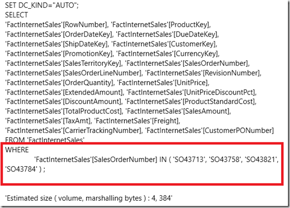
The trouble with this approach is that is that it can be very slow. Running a trace in DAX Studio for the query above reveals the problem:

The presence of CallbackDataID shows that the Storage Engine is calling the Formula Engine to handle the use of PathContains() in the filter, and this is often a cause of poor query performance. However back when I wrote the post the only alternative was, as Chris Koester points out here, to dynamically generate the entire DAX query as an SSRS expression and that is very painful to do.

The good news is that recent changes in DAX mean that there is another way to tackle this problem that can give much better performance. Here’s an example of this new approach:

EVALUATE
VAR OrderList = "SO43713|SO43758|SO43784|SO43821"
VAR OrderCount =
    PATHLENGTH ( OrderList )
VAR NumberTable =
    GENERATESERIES ( 1, OrderCount, 1 )
VAR OrderTable =
    GENERATE (
        NumberTable,
        VAR CurrentKey = [Value]
        RETURN
            ROW ( "Key", PATHITEM ( OrderList, CurrentKey ) )
    )
VAR GetKeyColumn =
    SELECTCOLUMNS ( OrderTable, "Key", [Key] )
VAR FilterTable =
    TREATAS ( GetKeyColumn, FactInternetSales[SalesOrderNumber] )
RETURN
    CALCULATETABLE ( FactInternetSales, FilterTable )

Broken down variable by variable, here’s how it works:

1. OrderList is the pipe-delimited list of key values passed from SSRS
2. OrderCount uses the PathLength() DAX function to find the number of parameter values in this list
3. NumberTable uses the GenerateSeries() function to create a table of numbers with one row for each number between 1 and the number of parameter values in the list
4. OrderTable uses the trick Marco describes here to iterate over NumberTable and, for each row, uses the PathItem() function to return one parameter value from the list for each row in the able
5. GetKeyColumn uses the SelectColumns() DAX function to only return the column from OrderTable that contains the parameter values
6. FilterTable uses the TreatAs() DAX function to take the table of values returned by GetKeyColumn and treat them as values in the FactInternetSales[SalesOrderNumber] column
7. Finally, the query returns the contents of the FactInternetSales table filtered by the values in FilterTable using the CalculateTable() DAX function

There’s a lot of extra code here and in some cases you may find that performance with smaller data volumes is worse as a result, but in this particular case the new approach is twice as fast at the old one. There’s certainly no CallBackDataID:

The recent blog post on the Analysis Services team blog about new memory options contained information about some very interesting functionality that has just been added. The first of the new features I decided to try was the RowsetSerializationLimit server property, which restricts the number of rows returned by a query and which is intended to stop rogue users running queries that return very large amounts of data. It certainly works but there are two things to point out about it that aren’t immediately obvious.

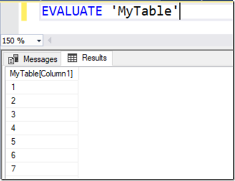
First of all, an example of it in action. In Azure Analysis Services, using a database that contains one very simple table with one column and 5000 rows, the following DAX query returns all 5000 rows from the table:

EVALUATE 'MyTable'

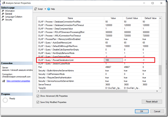
To change the RowsetSerializationLimit server property, open SQL Server Management Studio, right-click on your server name in the Object Explorer pane and select Properties. Then go to the General page, check the Show Advanced (All) Properties box, and you’ll see the property listed under OLAP\Query\RowsetSerializationLimit:

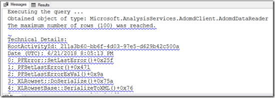
The default value is –1, meaning no limit is placed on the number of rows returned by a rowset. Changing it to 100 and then running the above query results in the following error:

Executing the query …
Obtained object of type: Microsoft.AnalysisServices.AdomdClient.AdomdDataReader
The maximum number of rows (100) was reached.

A query that returns less than 99 rows, for example

EVALUATE TOPN(99,'MyTable')

…is ok though.

The important thing to understand is that although this applies to both DAX and MDX queries, it only applies to queries that are returned as rowsets (a tabular format) and not as cellsets (a multidimensional format). Most client tools that generate MDX, including Excel, use cellsets so this property will not apply to them unfortunately.

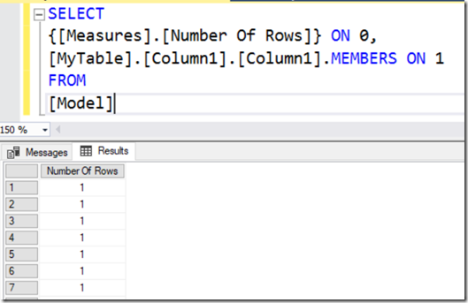
For example, the following MDX query run from a SQL Server Management Studio MDX query window (which also returns a cellset) on the same database runs ok and returns 5000 rows:

SELECT
{[Measures].[Number Of Rows]} ON 0,
[MyTable].[Column1].[Column1].MEMBERS ON 1
FROM
[Model]

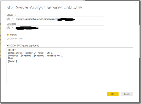
However the same query run from Power BI Desktop to import data from the same database:

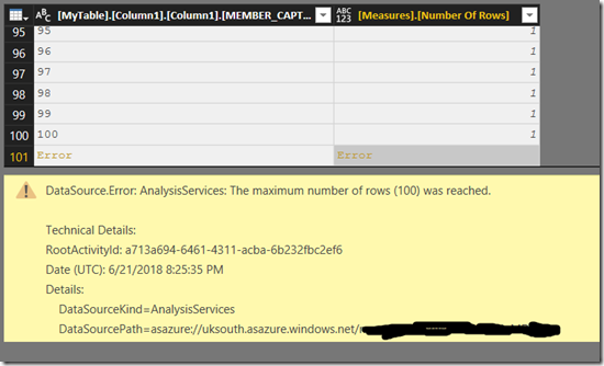
…runs, but returns only 100 rows and then an error:

Something else to point out is that this applies to all queries that return rowsets, even Discover requests and DMV queries. As a result, setting this property to a very low value can cause problems in tools like SQL Server Management Studio: for example if you set the property to 10 and you had 11 tables in a database, you would see an error when you tried to expand the Tables node of a database in the Object Explorer pane!

Even though this property only applies to rowsets I think it’s still going to be very useful, especially in scenarios where Power BI Desktop users are importing vast amounts of data from Analysis Services and causing major problems on the server.

Following on from my post the other week about the new RowsetSerializationLimit server property, I thought it would be a good idea to write about why the new IsAvailableInMDX property (announced in the same blog post) is so important. In fact, I would say that everyone using Analysis Services Tabular 2017 (CU7 or higher) or Azure Analysis Services should spend some time investigating it because the potential benefits in terms of reduced memory usage and faster processing times are significant, especially for larger models.

First of all, what does it actually do? As the blog post says, it allows you to stop attribute hierarchies from being built on columns when you don’t need them. But what are attribute hierarchies? They are structures that are used only when you are querying your Tabular model using MDX; Excel PivotTables, for example, generate MDX queries when they are connected to Analysis Services Tabular whereas Power BI always generates DAX queries. An attribute hierarchy allows a column on a table to be used on the rows or columns axis of an MDX query, and in Excel that means you will be able to drag that field onto the rows or columns area of a PivotTable. Attribute hierarchies are used by some DAX functionality too – for example the TreatAs() function (at least for now) needs them to be present to work. Frustratingly, the DAX functionality that does need attribute hierarchies is not documented.

To give you an example, consider a Tabular model that contains a table with three columns, Product, Customer and Sales, and a measure that sums up the values in the Sales column.

I can query this Tabular model in Power BI, for example by creating a Matrix visualisation:

I can also get the same values out using an Excel PivotTable:

Now the reason I can create this PivotTable is that Analysis Services Tabular has created attribute hierarchies on the Customer and Product columns. However, the important thing to understand is that Analysis Services Tabular creates attribute hierarchies on every column on every table by default, including the Sales column. This allows me to create a PivotTable like this, with the distinct values from Sales on the rows of the PivotTable:

You’re probably thinking, why would I ever want to use Sales – a measure column – like this? And the answer is you probably wouldn’t, even though Tabular allows this by default. What’s more, building the attribute hierarchy for Sales makes processing slower and the resulting hierarchy uses memory, so all this comes as a cost. The IsAvailableInMDX property is therefore very useful because it allows you to stop attribute hierarchies from being built on columns like Sales where they serve no real purpose.

Unfortunately at the time of writing SSDT doesn’t allow you to set the IsAvailableInMDX property but the good news is that the latest versions of Tabular Editor do:

Setting IsAvailableInMDX to false for the Sales field has no impact at all in Power BI, so long as you are not using functionality like TreatAs() that needs it. In Excel, it just means that it is no longer possible to drag Sales onto rows or columns in a PivotTable – the Sales Amount measure still works:

As a result, there are two recommendations that can be made:

• If you are not using any client tools that generate MDX queries (such as Excel) or you want to prevent your users from using them, and you can be sure that it does not affect any of your existing Power BI reports or DAX calculations, you can set IsAvailableInMDX to false on every column of every table
• If you are using client tools that generate MDX you can still probably set IsAvailableInMDX to false on every measure column and not lose any important functionality

How much of an impact will doing this have on processing times and memory usage? It depends, but it could be a lot. The anecdotal evidence on Twitter is promising:

I did my own (not particularly scientific) test using a table with five million rows and ten columns, each of which contained the integers between one and five million. Here’s the M query to generate such a table without the need for an external data source:

let
    Source =
	Table.FromColumns(
		List.Repeat(
			{{1..5000000}},
			10
		)
	),
    #"Changed Type" =
	Table.TransformColumnTypes(
		Source,
		List.Transform(
			Table.ColumnNames(Source),
			each {_, Int64.Type}
		)
	)
in
    #"Changed Type"

On my laptop, with IsAvailableInMDX set to true for all ten columns, a full process on this table took around 105 seconds and the table size reported by Vertipaq Analyzer was 381MB. After changing IsAvailableInMDX to false for all ten columns, the time for a full process went down to around 81 seconds and the table size was down to 191MB.

In summary, this is one of those seemingly obscure technical changes that turns out to be way more useful than you might think. If you test out setting IsAvailableInMDX on your Tabular model, please leave a comment letting me know what kind of impact it had!

[Thanks to Daniel Otykier for providing a lot of information for this post]

While I was playing around with the new release (August 2018) of Power BI Desktop I noticed there was an undocumented change: similar to the OData improvements I blogged about here, there is a new option in the AnalysisServices.Database() and AnalysisServices.Databases() M functions that turns on a newer version of the MDX generation layer used by the Power Query engine. Like the OData improvements it is an option called Implementation=”2.0”, used like this:

AnalysisServices.Databases(
	"localhost", 
	[
		TypedMeasureColumns=true, 
		Implementation="2.0"
	]
)

…and also, as with the OData improvements, you will need to manually edit any existing M queries to take advantage of this.

In fact first heard about this option in a comment on this blog post back in January, but as I was told by the dev team that it hadn’t been tested properly I didn’t blog about it. However as it is now set by default in the M code generated by the Power Query Editor, I guess it’s ready for production use. I’m told it should improve the performance of M queries that import data from Analysis Services – and I would be very interested to hear from anyone who tests this about how much of an improvement they see.

I’ve done a little bit of testing myself and I can see there are indeed some differences in the MDX generated. For example, I created an M query that connected to the Adventure Works DW database and returned all combinations of customer and day name where the Internet Sales Amount measure is greater than 100. In the old version of the MDX generation layer (ie without Implementation=”2.0” set) the following MDX query is generated:

SELECT
    {
        [Measures].[Internet Sales Amount]
    }ON 0,
    SUBSET(
        NONEMPTY(
            CROSSJOIN(
                [Date].[Day Name].[Day Name].ALLMEMBERS,
                [Customer].[Customer].[Customer].ALLMEMBERS
            ),
            {
                [Measures].[Internet Sales Amount]
            }
        ),
        4096
    )
    PROPERTIES MEMBER_CAPTION, MEMBER_UNIQUE_NAME ON 1
FROM(
    SELECT
        FILTER(
            CROSSJOIN(
                [Date].[Day Name].[Day Name].ALLMEMBERS,
                [Customer].[Customer].[Customer].ALLMEMBERS
            ),
            (
                NOT((
                    ISEMPTY(
                        [Measures].[Internet Sales Amount]
                    )
                OR
                    ISEMPTY(
                        100
                    )
                ))
            AND
                ([Measures].[Internet Sales Amount] > 100)
            )
        )ON 0
    FROM [Adventure Works]
)CELL PROPERTIES VALUE

However with the Implementation=”2.0” option set, the following query is generated:

SELECT
    {
        [Measures].[Internet Sales Amount]
    }ON 0,
    SUBSET(
        NONEMPTY(
            FILTER(
                CROSSJOIN(
                    [Date].[Day Name].[Day Name].ALLMEMBERS,
                    [Customer].[Customer].[Customer].ALLMEMBERS
                ),
                (
                    NOT(ISEMPTY(
                        [Measures].[Internet Sales Amount]
                    ))
                AND
                    ([Measures].[Internet Sales Amount] > 100)
                )
            ),
            {
                [Measures].[Internet Sales Amount]
            }
        ),
        4096
    )
    PROPERTIES MEMBER_CAPTION, MEMBER_UNIQUE_NAME ON 1
FROM [Adventure Works] CELL PROPERTIES VALUE

The difference between the two is that the first query uses a subselect to do the filtering whereas the second does not; subselects in MDX are not necessarily bad, but I generally try to avoid using them unless I need to. There may be other differences in the way the MDX is generated in the new version but I haven’t had a chance to do any detailed testing.

I  don’t like writing reviews of books or products here on my blog for a couple of reasons, the main one being that I don’t usually have the time to read/test/understand something properly so I can write a thorough review. That said I do get sent a lot of free books and evaluation licences for products that deserve a wider audience, so I thought I would write a post rounding up some of them along with a few thoughts of my own.

Custom Visuals

One of the most interesting questions related to Power BI is whether third-party software companies will be able to build businesses selling extensions to it. The most obvious way that Power BI can be extended is through custom visuals and there are several companies that have paid-for (as opposed to free) custom visuals. Zebra BI is one such company and I’ve been really impressed by what they have produced for visualising financial data:

I also saw recently that OKViz (part of the Marco and Alberto/SQLBI family) now have a paid-for version of their excellent Smart Filter visual with some premium features – see here for more details; similarly new features in Klaus Birringer’s Ultimate Waterfall and Ultimate Decomposition Tree visuals are only available in the paid version.

I know many Power BI users who use custom visuals have suffered with various bugs and limitations in functionality over the past few users, and I think buying commercial custom visuals rather than relying on free equivalents is one way of dealing with reliability and support problems. It’s certainly in Microsoft’s interests to have a thriving partner community in this space given that flashy visuals are a major selling point of the product. But will Power BI users want to pay for visuals when so much is available out of the box for free, especially when the cost of the visuals seems relatively high when compared to the overall cost of Power BI? I guess we’ll see.

Custom Connectors

A lot of what I’ve just said about custom visuals also applies to custom connectors, although custom connectors are a lot less mature (at the time of writing, support for custom connectors in the on-premises gateway is still in preview). However I was pleased to see this announcement from CData software that they now have over 100 custom connectors available for Power BI. It looks like what they have done is wrapped their existing ODBC providers, and as a result some of their connectors are for sources that are already available in Power BI, but even so there are a lot of new data sources here.

Incidentally, I got very, very excited when I realised that the CData connectors for Excel and Excel Online supported DirectQuery mode as well as import mode. Why, I hear you ask? Well, just think about a planning/budgeting solution where users can enter data into an Excel spreadsheet and when the numbers change in Excel, the numbers change in Power BI too; think also how this could work with Composite Models. I tried this with CData’s Excel on-premises connector and unfortunately it returned errors when the source Excel worksheet was open; I did get it to work with the Excel Online connector but it was painfully slow, even with a small amount of data. If I can get it to work better (and I may be missing some optimisations within the connector) I’ll blog about it.

Books

One of the few Power BI-related books that have been published recently is Phil Seamark’s “Beginning DAX with Power BI”. He was kind enough to send me a review copy; it’s a good introduction to the subject and I particularly like the way he introduces DAX variables early one. Definitely worth a look if you’re just starting to learn DAX.

I was also sent a copy of a slightly older book, David Parker’s “Mastering Data Visualization with Visio 2016”. David knows pretty much all there is to know about using Visio for BI (his blog is great) and while this book doesn’t cover the most exciting new development in this area – the Visio custom visual for Power BI – if you want to learn all the advanced features of Visio that you could take advantage of in Power BI then this is the book to get.

Other Products

I’ve been a big fan of SentryOne’s SSAS monitoring tool, BI Sentry, for years now but up until recently it only supported SSAS Multidimensional. It now supports SSAS Tabular too (details here), and it looks like SentryOne have done a great job of adapting it to the specific needs of the Tabular engine. I always advise my SSAS customers to invest in some kind of monitoring solution because it makes the job of detecting and solving issues like poor query performance so much easier, and to be honest BI Sentry is better than anything you would be able to build yourself.

Moving onto Power BI, if you need to generate documentation for your Power BI datasets and reports check out Power BI Documenter; the August release looks like it has some cool new features. Alternatively the latest release of Power BI Helper also allows you to generate documentation as well as lots of other useful stuff.

Something that hasn’t been properly released yet, but will be incredibly useful when it is, is MAQ Software’s Application Lifecycle Management Toolkit for Power BI. Closely related to BISM Normalizer, it will allow you to compare two Power BI datasets, merge changes, deploy only parts of a dataset (for example individual measures), and deploy to multiple datasets – all of which are things Power BI developers have been crying out for.

Last of all, the guys at DevScope also have a new(ish) product out, Power BI Robots, which automatically takes screenshots of Power BI reports and dashboards and can deliver them to various destinations such as email address and SharePoint. I haven’t looked at it yet but it seems like it could have a lot of interesting uses.

Recently I was working on an MDX calculation that calculated a value at a low granularity and aggregated the result – basically what I described in my blog post here. Here’s a simplified version of the calculation written on a cube built from Adventure Works data running on my local SSAS 2017 MD instance:

SCOPE([Measures].[Tax Amount]);
    SCOPE(
	[Customer].[Customer].[Customer].MEMBERS, 
	[Date].[Date].[Date].MEMBERS, 
	[Product].[Product].[Product].MEMBERS);
        THIS = [Measures].[Sales Amount]*0.08;
    END SCOPE;
END SCOPE;

All it does is take the value of the Sales Amount measure at the lowest granularities of the Customer, Date and Product dimensions, multiply it by 0.08 to find a tax value, and because [Tax Amount] is a real, non-calculated measure, the result of the calculation aggregates up through the cube. [I know that I don’t have to aggregate the result of this specific calculation but remember that this is a simplified example – in the real case I did have to write the calculation using Scope statements – and anyway the best way of handling a basic multiplication like this would be with a measure expression]

The performance was sub-second for my test query and I was happy, but then I realised that the same tax rate was being used in other calculations and may change in the future, so I thought I would store the value 0.08 in a calculated measure:

CREATE MEMBER CURRENTCUBE.[Measures].[Tax Rate] AS  
0.08;

SCOPE([Measures].[Tax Amount]);
    SCOPE(
	[Customer].[Customer].[Customer].MEMBERS, 
	[Date].[Date].[Date].MEMBERS, 
	[Product].[Product].[Product].MEMBERS);
        THIS = [Measures].[Sales Amount]*[Measures].[Tax Rate];
    END SCOPE;
END SCOPE;

Surely a simple change? But no, as soon as I did this my query ran for several minutes and memory usage went through the roof until the query was automatically cancelled:

Clearly the SSAS MD Formula Engine could optimise the version with the hard-coded constant value but could not optimise the version with the calculated measure. There was nothing in Profiler to indicate the calculation was being evaluated in cell-by-cell mode though.

So I tried another variation:

CREATE MEMBER CURRENTCUBE.[Measures].[Tax Rate] AS  
IIF([Measures].[Sales Amount]=0, NULL, 0.08);

SCOPE([Measures].[Tax Amount]);
    SCOPE(
	[Customer].[Customer].[Customer].MEMBERS, 
	[Date].[Date].[Date].MEMBERS, 
	[Product].[Product].[Product].MEMBERS);
        THIS = [Measures].[Sales Amount]*[Measures].[Tax Rate];
    END SCOPE;
END SCOPE;

This time the memory usage was completely flat but the query was still so slow had to be cancelled. Next, I thought I’d try setting the NON_EMPTY_BEHAVIOR property:

CREATE MEMBER CURRENTCUBE.[Measures].[Tax Rate] AS  
0.08
, NON_EMPTY_BEHAVIOR = [Measures].[Sales Amount];

SCOPE([Measures].[Tax Amount]);
    SCOPE(
	[Customer].[Customer].[Customer].MEMBERS, 
	[Date].[Date].[Date].MEMBERS, 
	[Product].[Product].[Product].MEMBERS);
        THIS = [Measures].[Sales Amount]*[Measures].[Tax Rate];
    END SCOPE;
END SCOPE;

And guess what? The query went back to being sub-second. Strange. Now the NON_EMPTY_BEHAVIOR property is very dangerous and this is a clear example of how it should not be set – the expression 0.08 is never going to return an empty value, regardless of the value of the [Sales Amount] measure. As a result I would be very wary of using this trick in production in case it ended up returning inconsistent results. It’s also worth noting that the following calculation, which is a correct use of NON_EMPTY_BEHAVIOR, is as slow as the other examples above:

CREATE MEMBER CURRENTCUBE.[Measures].[Tax Rate] AS  
IIF([Measures].[Sales Amount]=0, NULL, 0.08)
, NON_EMPTY_BEHAVIOR = [Measures].[Sales Amount];

Finally I created a dummy table in my DSV with one row and one column to hold the 0.08 value, and then created a real, non-calculated measure from the column. When I used this measure in my calculation then performance of my test query was also sub-second.

So, to sum up, it looks like hard-coding constant values in calculated measures is a bad idea, at least in cases like this, and either using the values themselves in your MDX calculations or creating a table and non-calculated measure specifically to hold the value is better for performance.

The big news in the world of Excel right now is the introduction of dynamic arrays. They’re only available in the Office 365 click-to-run version of Excel and, at the time of writing, only available to people on the Office Insiders programme, but eventually they’ll be available to anyone running Excel for Office 365 on their desktop. There are already lots of blog posts about them including this overview by Jon Acampora, and you probably also want to download Bill Jelen’s detailed mini-book on them here which is free for the rest of 2018. Now I’m not an Excel expert by any stretch of the imagination but I’m as excited as anyone else about them because they will be incredibly useful for anyone building reports using Excel cube functions against Analysis Services, the Excel Data Model/Power Pivot and Power BI. Bill Jelen’s book has a short section on this subject but the possibilities are limitless…

Here’s one example of how they can be used. A while ago I blogged about how to use a regular array formula and the TextJoin() Excel function to get all the selected items from a slicer. Dynamic arrays make this problem much easier to solve. Take the following table loaded into the Excel Data Model:

Now, say you have a PivotTable built from this and a slicer (called Slicer_Fruit) connected to it:

It’s possible to use the CubeSet() function to get the set of selected items in a slicer using the following formula:

=CUBESET("ThisWorkbookDataModel",Slicer_Fruit,"Slicer Set")

Assuming this formula is in cell H1, you can then get the number of items in this set using CubeSetCount():

=CUBESETCOUNT($H$1)

Assuming this is in cell H2, all you need to do to get a comma-delimited list of all the selected items in the slicer via this set is:

=
 TEXTJOIN(
  ", ", 
  TRUE, 
  CUBERANKEDMEMBER(
   "ThisWorkbookDataModel",
   $H$1, 
   SEQUENCE($H$2,1)
  )
 )

Here it is in action:

It works as follows:

• The new Sequence() function is used to create a dynamic array of numbers from one to the number returned by the CubeSetCount() function.
• The CubeRankedMember() gets the name of each of the items in the set using the numbers returned by Sequence()
• TextJoin() then concatenates all of the names returned by CubeRankedMember() into a single comma-delimited list.

You can download the sample workbook here (remember it will only work if you have a version of Excel installed that includes dynamic arrays!).

I’m at the PASS Summit this week, and in this morning’s keynote there was a demo of the newly-released Azure Data Studio  – a modern, cross-platform tool for managing and querying SQL Server, Azure SQL Database and other Azure data services (it’s carefully described as “complementary to” SQL Server Management Studio rather than a replacement for it; this blog post has a detailed discussion of this question).

This video is provides a good, short overview of what it is:

I think it’s pretty cool, BUT… it doesn’t support Analysis Services. I had a moan about this and the generally poor state of Analysis Services tooling on Twitter, was invited to meet some of the developers and was told that if enough people request Analysis Services support it might happen.

What would support for Analysis Services involve? The following springs to mind:

• I’d like to be able to connect to and manage Analysis Services Multidimensional and Tabular on-premises and Azure Analysis Services; if that’s too ambitious I could settle for supporting only Analysis Services Tabular 2016+ and Azure Analysis Services.
• Since we will soon be able to connect to a Power BI Premium capacity as if it was an Analysis Services instance via XMLA endpoints, I would want to be able to connect to Power BI Premium capacity too.
• I’d want to be able to run DAX and M queries, and ideally MDX queries too.
• I would also want to be able to work with ASSL and TMSL for scripting and editing objects.
• Azure Data Studio has a Profiler extension that works on xEvents; it would be great if that worked with Analysis Services xEvents too.
• DAX and M Jupyter notebooks would be really useful!
• It would make sense for some of the functionality of existing tools like DAX Studio and BISM Normalizer being turned into extensions.

If you want to see Analysis Services support in Azure Data Studio, go to the following issue on the Azure Data Studio GitHub repository:

https://github.com/Microsoft/azuredatastudio/issues/1026

…and click the thumbs-up icon on the first post:

Let’s make our voices heard!

Today marks the 20th birthday of Analysis Services: it was released (as OLAP Services) on November 16th 1998. There’s a celebratory blog post and video over on the Power BI blog here:

https://powerbi.microsoft.com/en-us/blog/analysis-services-is-20-years-old/

I’m one of the interviewees on the video, and in it I tell the story of my involvement with Analysis Services and MDX – I’ve been working with it almost full-time for a little over 20 years, right from the first betas. I’ve enjoyed every minute of it, and I’d like to take the opportunity here to thank all the people who have helped me over the years at IMS Health, Microsoft Consulting Switzerland, in the SSAS and Power BI community, and in my career as an independent consultant and trainer. If you had told me in 1998 that I would still be making a living with this product (even still writing some MDX) I’m not sure I would have believed you.

Finally, if your Bingling skills have failed you, here’s the OLAP Jokes post that is mentioned in the birthday video:

https://blog.crossjoin.co.uk/2005/08/25/olap-jokes/

It was for many years the most popular post on my blog. I should point out that I didn’t write all those jokes: my colleagues at the time, Jon Axon and Colin Hardie, deserve some of the blame too.

With the release of CTP 2.3 of SQL Server 2019 today there was big news for Analysis Services Tabular developers: Calculation Groups. You can read all about them in detail in this blog post:

https://blogs.msdn.microsoft.com/analysisservices/2019/03/01/whats-new-for-sql-server-2019-analysis-services-ctp-2-3/

In my opinion this is the most important new feature in DAX since… well, forever. It allows you to create a new type of calculation – which in most cases will be a time intelligence like a year-to-date or a previous period growth – that can be applied to multiple measures; basically the same thing that we have been doing in SSAS Multidimensional for years with the time utility/shell/date tool dimension technique. It’s certainly going to solve a lot of problems for a lot of SSAS Tabular implementations, many of which have hundreds or even thousands of measures for every combination of base measure and calculation type needed.

I’m not going to repeat any of the detailed technical information in the blog post here, though. Instead the point I want to make is that this is very big news for SSAS Multidimensional users too. In the past couple of years many people who have existing SSAS Multidimensional implementations have thought about migrating to SSAS Tabular so they can take advantage of its new features or move to the cloud, and indeed many of them have already migrated successfully. However, up to now, the biggest blocker for those wanting to migrate from Multidimensional to Tabular has been the fact that some complex calculations that can be expressed in MDX cannot be recreated (or recreated easily and efficiently) in DAX, because DAX has not had an equivalent of calculated members not on the Measures dimension or the MDX SCOPE statement.

Calculation groups do not remove this roadblock completely, but they do remove the roadblock for a large group of existing SSAS Multidimensional users whose only complex calculation requirement is a time utility/shell/date tool dimension. As a result these SSAS Multidimensional users will now be able to migrate to SSAS Tabular 2019, Azure Analysis Services or Power BI if they want to. Only those people who have more exotic uses for calculated members not on the Measures dimension (which are not very common at all) and those who use SCOPE statements (a larger group – many people working with financial data use SCOPE statements heavily) will find that Multidimensional is still the correct platform for them.

SQLBits is one of the best Microsoft data platform conferences around, and last week’s event in Manchester was particularly good. As usual, videos of almost all of the sessions are available for everyone to view for free online (no registration required) here:

https://sqlbits.com/content/Event18

There were lots of Power BI and Analysis Services related sessions, so I thought I’d call out a few:

• If you’re interested in the new calculation groups feature in SSAS 2019 that I blogged about last week, you should definitely watch Christian Wade’s two-part session here and here (part two has all the juicy details in), which also gives some details about other upcoming features such as XMLA endpoints. Kasper’s session here covers a lot of the same topics.
• There’s more insight into Microsoft’s Power BI roadmap and thinking in the Q&A session with Christian, Kasper and Adam here
• Marco and Alberto always do great sessions, and Alberto’s session on Aggregations here and Marco’s session on many-to-many relationships here are up to their usual high standards.
• My session on Power BI Dataflows here sums up my current thoughts about them.

Of course there’s lots more there (more than I have had a chance to watch) so let me know if there are other sessions that are good!

An interesting – if obscure – fact I learned recently is that a small number of DAX functions such as Median() do not work on tables with more than 2 billion rows in Analysis Services Tabular, Azure AS and Power BI.

It’s quite easy to reproduce in Power BI. The following M expression returns a table with two billion and four rows:

let
    Source = 
    List.Repeat(
        {1,2,3,4},
        500000001
        ),
    #"Converted to Table" = 
    Table.FromList(
        Source, 
        Splitter.SplitByNothing(), 
        null, 
        null, 
        ExtraValues.Error
        ),
    #"Changed Type" = 
    Table.TransformColumnTypes(
        #"Converted to Table",
        {{"Column1", Int64.Type}}
        )
in
    #"Changed Type"

It takes some time to load this table  – around twenty minutes – but because there are only four distinct values in the table the resulting .pbix file is only 31KB thanks to the way Power BI compresses data.

If you load this table into your dataset, call it VeryBigTable and create the following measure:

Median Test = MEDIAN(VeryBigTable[Column1])

…and use the measure in a visual, you’ll see the following error:

The current query cannot be evaluated for the ‘VeryBigTable (42)’ table, because the table contains more than two billion rows.

What’s more, the error will always occur even if you apply a filter to the table that returns less than two billion rows. The same problem occurs with some other functions, such as Percentile(), but it’s worth pointing out that the vast majority of DAX functions work as normal with tables with more than two billion rows – for example, in the pbix file used here the Sum() and CountRows() functions not only work fine but return instantly.

Luckily, in the case of the Median() function, there is an easy workaround because you can calculate a median in other ways such as the one described on the DAX Patterns site here. The code is a lot more verbose but it works on a 2 billion+ row table.

There are a lot of great community-developed tools out there for Analysis Services developers to use (BI Developer Extensions, DAX Studio, Tabular Editor, Analysis Services Query Analyzer to name a few) and they have saved me vast amounts of time and effort over the years. When I joined Microsoft last month I came across one which I had never seen before but which is nevertheless quite mature and feature-rich: the SSAS Diagnostics Tool or SSASDiag for short. It’s available on GitHub here:
https://github.com/ssasdiag/SSASDiag

…and you can read the documentation here:
https://github.com/ssasdiag/SSASDiag/wiki/SSAS-Diagnostics—Analysis

It’s an open source tool developed by the people who support Analysis Services here at Microsoft and is intended to help them collect and analyse the information they need to troubleshoot on-premises SSAS  issues, but it’s available for anyone to use. I haven’t had a chance to take a proper look at it yet myself, unfortunately, but I thought it would be interesting for any SSAS fans out there to check out.

[Thanks to Jon Burchel for providing all the background information for this post]

In Shabnam Watson’s recent blog post on a bug she found when trying to create a Live connection from Power BI to Analysis Services she mentioned that the AutoSetDefaultInitialCatalog server property could be used to solve her problem. This piqued my interested because I’d seen this property but had no idea what it did exactly or why it was there. Luckily, now I work for Microsoft, it’s even easier for me to find out about things like this from the dev team and Akshai Mirchandani was able to help.

First of all, what does it do? The documentation on this property has just been added here, and this is what it says:

AutoSetDefaultInitialCatalog
A Boolean property. When set to true, new client connections automatically default to the first catalog (database) the user has permissions to connect to.
When set to false, no initial catalog is specified. Clients must select a default catalog prior to running queries or discover operations against a database on the server. If no default catalog is specified, an error is returned. If Initial Catalog property is specified in the connection string, the default catalog will be applied from this property.

The default value for this property is true.

Let me illustrate what this means. Say you have an instance of Analysis Services (in this case it’s Tabular, but it could be Multidimensional) with two databases on it:

I’ve expanded the Roles tab for each database reasons that will become clear later.

Next, let’s say you run a simple trace on this server looking at the Discover End and Session Initialize events:

…and while this trace is running, you open up SQL Server Management Studio and connect to the SSAS instance. Here’s what you see in Profiler:

Now, just to be clear, all I did was open up SQL Server Management Studio and connect to the instance. I did not open up a DAX query window or anything like that; all that happened was the list of databases on the instance was displayed in the Object Explorer pane.

The interesting thing to notice from the trace above is that when I did that there are five Session Initialize events and even though the Database column in Profiler is blank, you can see from the list of role names in the TextData column that in each case a connection has been made to the Adventure Works Internet Sales database.

This is because when you open a connection to Analysis Services and do not set the Initial Catalog connection string property, what happens is that you will get a connection to the default database on the instance. Which database is the default? It’s just the first database that the user has permission to access on the instance, which is a bit random.

This happens at other times too. Let’s say you right click on the EmptyDB database and process it in SQL Management Studio:

Here’s what I see in Profiler:

In this case there are three connections to the default database, Adventure Works Internet Sales, when the database I am processing is EmptyDB!

Most of the time these unnecessary connections have no impact at all but sometimes they can cause problems such as the ones Shabnam describes in her blog post. For example:

• It can cause performance problems, because there is an overhead to opening a connection – for example roles are evaluated when a connection is opened
• Monitoring and auditing gets complicated because, as you can see from the traces above, there are a whole lot of connections to the default database taking place that you aren’t expecting
• Most importantly, when a connection is opened a read-commit lock is acquired on that database and in a few rare cases this can cause deadlocks and other locking-related issues

This is why the AutoSetDefaultInitialCatalog server property was introduced. With this server property set to False, when you open a connection to SSAS with no Initial Catalog set, then you get a connection with no database set. You can find this server property in SQL Server Management Studio in the Analysis Server properties dialog (which you can find by right-clicking on your instance name, selecting Properties, and going to the General tab) and checking the Advanced (All) Properties box.

With AutoSetDefaultInitialCatalog set to False, here’s what Profiler shows when I rerun my original test of connecting to SQL Server Management Studio:

Note that there are now no Session Initialize events now.

Here’s what opening up a new MDX query window in SQL Management Studio shows with AutoSetDefaultInitialCatalog set to False if you don’t explicitly set a database when you connect:

Note the empty database dropdown box on the toolbar and the “Error loading metadata: No cubes were found” error message shown in the Metadata pane.

So why didn’t the dev team set AutoSetDefaultInitialCatalog to False by default on new instances? The problem with doing this is that it is a potential breaking change that could cause errors in some client tools. I’m not aware of any specific cases where this might happen but if you did decide to change AutoSetDefaultInitialCatalog to False on your instance you would need to test thoroughly to make sure it didn’t break anything. My feeling is, though, it is probably a good idea to AutoSetDefaultInitialCatalog to False on production servers and do the appropriate testing just in case those unnecessary connections are causing problems.

Back in 2016 I wrote the following blog post about changes to the way Excel 365 generated MDX queries for PivotTables connected to Analysis Services, Power Pivot/the Excel Data Model and Power BI datasets:

https://blog.crossjoin.co.uk/2016/07/08/excel-2016-pivottable-mdx-changes-lead-to-big-query-performance-gains/

I know it sounds boring and not something you need to worry about but trust me, this is important – these changes solved the vast majority of Excel PivotTable performance problems that I encountered when I was a consultant so you should read the above post before continuing.

Unfortunately, earlier this year these changes had to be partially rolled back because in some rare cases the queries generated returned incorrect results; this means that you may find that values for subtotals and grand totals are again being returned even when they aren’t being displayed. The good news is that you should still be able to get the improved performance with a few minor tweaks.

Using the example from the previous post, a PivotTable connected to SSAS MD and the Adventure Works cube (the queries generated for SSAS Tabular, Power Pivot and Power BI may be slightly different and slightly better but the basic problem is the same), if you build the following in Excel:

…even though the subtotals in the PivotTable are not displayed in Excel, the MDX query generated by Excel not only returns them but also returns others that are not needed at all – in fact 36 rows (although the query returns them as columns) of data rather than the 13 rows that are displayed. Here’s a screenshot of the results returned when you run the MDX query in SQL Server Management Studio:

Any time you see a row or column containing an All Member (in this case All Customers or All Products) you know you are looking at a subtotal or grand total.

[NB The easiest way to get the MDX query generated by your PivotTable is to install the OLAP PivotTable Extensions add-in https://olappivottableextensions.github.io/]

In this case, to get an efficient query, you need to explicitly turn off subtotals and grand totals for the PivotTable in Excel:

In the PivotTable the only difference you’ll see is that the grand totals are now not displayed:

But the query generated now only returns the values that are actually needed, and as a result will be a lot more efficient and potentially a lot faster. In this case, the query now only returns the 12 rows of data displayed:

Even with subtotals and grand totals turned off there are still some cases where unwanted values will be returned. Take the following PivotTable, where I have used the Calendar hierarchy from the Date dimension on columns and filtered it so I only see the three months in Q1 CY 2012:

The MDX query generated by Excel requests requests four extra columns with subtotals and a grand total that aren’t displayed:

There is a fairly simple workaround though. By changing how the PivotTable is constructed – in this case by not putting a hierarchy on columns but just the Month Of Year attribute, then adding slicers for Calendar Year and Calendar Quarter to control which months are displayed – you can get an efficient query. This version of the PivotTable:

…results in this query being generated, which only returns the required values:

To sum up, then, if you have a PivotTable that seems a bit slow:

• Turn off subtotals and grand totals unless you really need to see them
• Look at the MDX query being generated by Excel and see if it is still returning unnecessary subtotals and grand totals, and if it is try rebuilding the PivotTable to get the same results in a different way (for example by not drilling down on hierarchies as in the last example) to get a more efficient query

[All the queries in this post were generated by Excel 365 version 1910 build 12130.20238]